effector

effector is an eXplainable AI package for tabular data. It:

explains any black-box model with global and regional effects: what each feature does, and where the average hides something
produces a report in one line: effector.explain(X, model) fits, ranks the features, hunts for subregions, and writes a single self-contained HTML page
offers an interactive API when you want the controls: five engines (PDP, d-PDP, ALE, RHALE, SHAP-DP), one verb set
is model agnostic: any callable numpy → numpy works, and adapters wrap scikit-learn, PyTorch, classifiers and DataFrame pipelines
is fast, for both global and regional methods: everything after the fit is free

📖 Documentation | 🚀 Quickstart | 🔧 API | 🏗 Examples

Installation

Effector requires Python 3.10+:

pip install effector

This installs a lightweight core (numpy, scipy, matplotlib, tqdm) that covers PDP, ALE, RHALE and their regional effects.

ShapDP needs the heavier shap/shapiq backends (which pull in numba, scikit-learn, pandas, ...). Install them only if you use that method:

pip install effector[shap]

Quickstart

(a) The inputs

A dataset as a numpy array, a model as a numpy → numpy callable, and, optionally, a schema so the explanation speaks your vocabulary:

import effector
from sklearn.ensemble import HistGradientBoostingRegressor

data = effector.datasets.BikeSharing()  # standardized numpy arrays
model = HistGradientBoostingRegressor(random_state=21).fit(data.x_train, data.y_train)
predict = effector.adapters.from_sklearn(model)  # a plain numpy -> numpy callable

schema = effector.Schema(
    feature_names=data.feature_names,
    feature_types=[
        "nominal", "nominal", "ordinal", "ordinal", "nominal", "nominal",
        "nominal", "ordinal", "continuous", "continuous", "continuous",
    ],
    category_names=[
        ["winter", "spring", "summer", "fall"],
        ["2011", "2012"],
        ["Jan", "Feb", "Mar", "Apr", "May", "Jun",
         "Jul", "Aug", "Sep", "Oct", "Nov", "Dec"],
        None,
        ["no", "yes"],
        ["Sun", "Mon", "Tue", "Wed", "Thu", "Fri", "Sat"],
        ["no", "yes"],
        ["clear", "mist", "light rain/snow", "heavy rain"],
        None, None, None,
    ],
    scale_x_list=[
        {"mean": data.x_train_mu[i], "std": data.x_train_std[i]}
        for i in range(data.x_train.shape[1])
    ],
    scale_y={"mean": data.y_train_mu, "std": data.y_train_std},
    target_name="bike-rentals",
)

📄 In depth: the input layer; pandas, sklearn, torch, classifiers, feature types, units.

(b) The one-liner

report = effector.explain(
    data.x_train, predict, y=data.y_train, schema=schema, nof_instances=5000
)

It fits once, ranks the features, hunts for subregions where the average is hiding something, keeps only the splits that pay for themselves, and opens with the one number worth having:

[effector] global effects   (GAM)  -> 72.3% of the model's variance
           regional effects (CALM) -> 92.0%

The result is a Report, a value you can export or print:

report.to_html("report.html")  # a single self-contained page; mail it, commit it
report.show()                  # the same story, as terminal tables

  ════════════════════════════════════════════════════════════════════════
  PDP report  ·  target: bike-rentals
  ════════════════════════════════════════════════════════════════════════

  DATA & MODEL
  ────────────────────────────────────────────────────────────────────────
    instances     5,000
    features      11  ·  5 nominal · 3 ordinal · 3 continuous
    model output  mean 188 · std 176 · range [-19.5, 948]
    model R²      0.960  (on this subsample)

  EXPLAINED VARIANCE
  ────────────────────────────────────────────────────────────────────────
    step         split on                 solo     ΔR²      R²       heter
    ──────────────────────────────────────────────────────────────────────
    GAM          (all features global)       —       —   72.3%           —
  + hr           temp, workingday, yr   +18.3%  +18.3%   90.6% 0.47 → 0.26
  + temp         hr, hum                 +2.4%   +1.4%   92.0% 0.22 → 0.19
    ──────────────────────────────────────────────────────────────────────
    FINAL                                                92.0%

  REJECTED SPLITS                                            min gain 1.0%
  ────────────────────────────────────────────────────────────────────────
    feature      split on                 solo     ΔR²    reason
    ──────────────────────────────────────────────────────────────────────
  ✗ yr           hr, workingday          +2.7%   -0.8%    redundant
  ✗ hum          hr, temp                +2.2%   +0.2%    below threshold
  ✗ weekday      hr, temp, yr            +0.4%   +0.2%    below threshold
  ✗ workingday   hr, yr                  +6.2%   -4.8%    redundant

    ✗ redundant: it would explain variance on its own (see solo),
      but the accepted splits already account for it.

  FEATURES                                ranked, in the selected snapshot
  ────────────────────────────────────────────────────────────────────────
    feature        importance                          heter      #regions
    ──────────────────────────────────────────────────────────────────────
    hr                 0.7273  ██████████████████     0.2608             4
    yr                 0.2271  ██████                 0.2088             1
    temp               0.2098  █████                  0.1874             4
    hum                0.0932  ██                     0.1221             1
    ──────────────────────────────────────────────────────────────────────
    the features above carry 82% of the total importance mass

(the accepted partition trees follow)

📄 In depth: the report; the explained variance ledger, the triage plane, the regional analysis, every knob of explain(...).

(c) The interactive API

The same engine, as a live handle you query as you go:

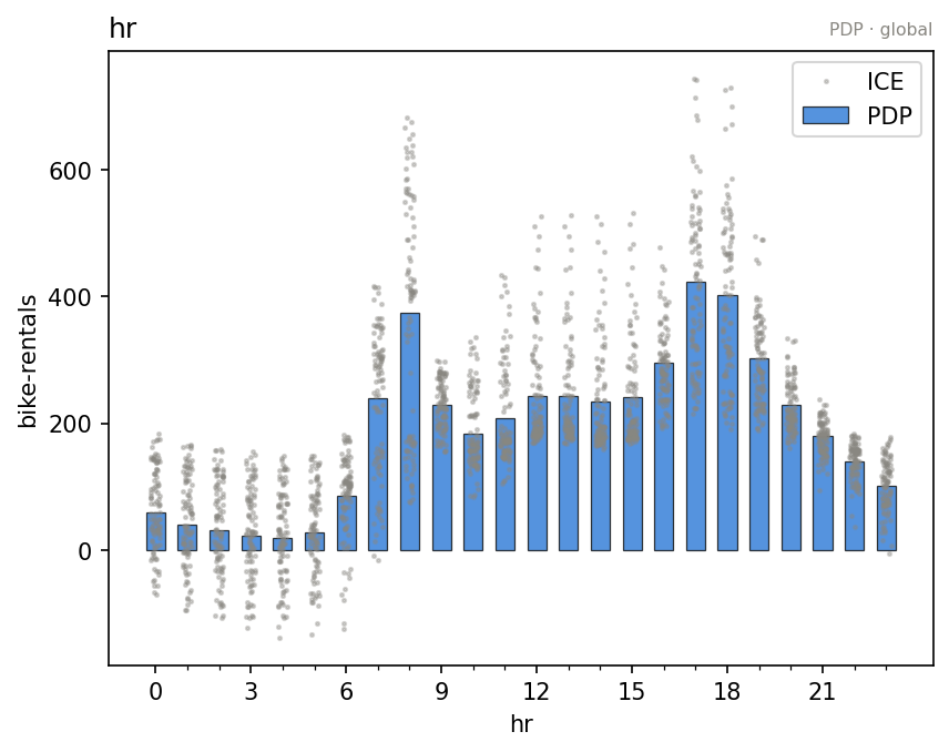
pdp = effector.PDP(data.x_train, predict, schema=schema, nof_instances=5000)

pdp.plot("hr")                        # the global effect, ICE curves behind it
pdp.heter_score("hr")                 # 0.47: the average hides a lot
partition = pdp.find_regions("hr")    # where is it hiding it?
partition.show()

Feature 3 - Full partition tree:
🌳 Full Tree Structure:
───────────────────────
hr 🔹 [id: 0 | heter: 0.47 | inst: 5000 | w: 1.00]
    workingday = no 🔹 [id: 1 | heter: 0.33 | inst: 1545 | w: 0.31]
        temp < 6.86 🔹 [id: 2 | heter: 0.22 | inst: 778 | w: 0.16]
        temp ≥ 6.86 🔹 [id: 3 | heter: 0.26 | inst: 767 | w: 0.15]
    workingday = yes 🔹 [id: 4 | heter: 0.34 | inst: 3455 | w: 0.69]
        yr = 2011 🔹 [id: 5 | heter: 0.23 | inst: 1720 | w: 0.34]
        yr = 2012 🔹 [id: 6 | heter: 0.31 | inst: 1735 | w: 0.35]
--------------------------------------------------
Feature 3 - Statistics per tree level:
🌳 Tree Summary:
─────────────────
Level 0🔹heter: 0.47
    Level 1🔹heter: 0.34 | 🔻0.13 (28.12%)
        Level 2🔹heter: 0.26 | 🔻0.08 (22.91%)

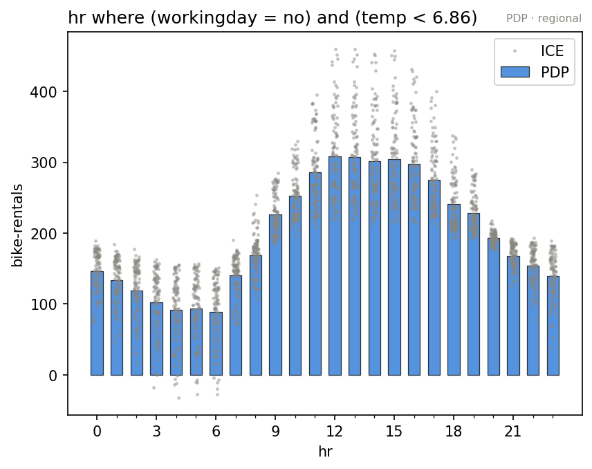
The effect of hr depends on workingday (commute peaks vs a midday plateau), and within each branch on temp and yr. Plot the effect inside a region:

partition.plot(2)  # hr, on non-working days, in the cold

Every verb answers one question:

verb	question it answers
`.plot(f)`	what does feature `f` do?
`.eval(f, xs)`	…as numbers, on my grid
`.importance(f)`	how much does `f` move the output?
`.heter_score(f)`	is the average hiding something?
`.find_regions(f)`	where is it hiding it?
`.select_regions()`	which splits actually earn their keep?
`.fit(features, **cfg)`	(optional) tune the method first

📄 In depth: the interactive API; construct and fit, customizing .fit(), plot, eval, scores, regions.

Documentation map

Start here:

What are global and regional effects: the concepts
effector's API: the whole API in 3 minutes
- (a) The input layer: numpy, models, adapters, the schema
- (b) effector's report: the one-liner, .show(), and the HTML page
- (c) The interactive API: the five engines, global and regional effects

Going deeper:

The mental model: the thinking behind the API; one engine, values not state, two entrances
Methods: the math reference: how each method defines the effect, its heterogeneity, and the two scalars
The design contract: the rules the API is built on, one breath each
Efficiency of global and regional methods: count the model calls

Supported Methods

Every method computes global effects, and regional effects via .find_regions(feature):

Method	Class	Reference	ML model	Speed
PDP	`PDP`	Friedman, 2001	any	fast for a small dataset
d-PDP	`DerPDP`	Goldstein et al., 2013	differentiable	fast for a small dataset
ALE	`ALE`	Apley & Zhu, 2020	any	fast
RHALE	`RHALE`	Gkolemis et al., 2023	differentiable	very fast
SHAP-DP	`ShapDP`	Lundberg & Lee, 2017	any	fast for a small dataset and a light model

Choosing a method

Three questions decide: is the dataset small (N < 10K) or large? Is the model light (< 0.1s per call) or heavy? Is it differentiable or not?

your case	use
small + light	any: `PDP`, `ALE`, `ShapDP`; plus `RHALE`, `DerPDP` if differentiable
small + heavy	`PDP`, `ALE`; plus `RHALE`, `DerPDP` if differentiable
large + differentiable	`RHALE`
large + non-differentiable	`ALE`

Citation

If you use effector, please cite it:

@misc{gkolemis2024effector,
  title={effector: A Python package for regional explanations},
  author={Vasilis Gkolemis et al.},
  year={2024},
  eprint={2404.02629},
  archivePrefix={arXiv},
  primaryClass={cs.LG}
}

Spotlight on `effector`

📚 Featured Publications

Gkolemis, Vasilis, et al.
"Fast and Accurate Regional Effect Plots for Automated Tabular Data Analysis."
Proceedings of the VLDB Endowment | ISSN 2150-8097

🎤 Talks & Presentations

LMU-IML Group Talk
Slides & Materials | LMU-IML Research
AIDAPT Plenary Meeting
Deep dive into effector
XAI World Conference 2024
Poster | Paper

🌍 Adoption & Collaborations

AIDAPT Project
Leveraging effector for explainable AI solutions.

🔍 Additional Resources

Medium Post
Effector: An eXplainability Library for Global and Regional Effects
Courses & Lists:
IML Course @ LMU
Awesome ML Interpretability
Awesome XAI
Best of ML Python

Papers that have inspired effector:

REPID: Regional Effects in Predictive Models
Herbinger et al., 2022 - Link
Decomposing Global Feature Effects Based on Feature Interactions
Herbinger et al., 2023 - Link
RHALE: Robust Heterogeneity-Aware Effects
Gkolemis Vasilis et al., 2023 - Link
DALE: Decomposing Global Feature Effects
Gkolemis Vasilis et al., 2023 - Link
Greedy Function Approximation: A Gradient Boosting Machine
Friedman, 2001 - Link
Visualizing Predictor Effects in Black-Box Models
Apley, 2016 - Link
SHAP: A Unified Approach to Model Interpretation
Lundberg & Lee, 2017 - Link
Regionally Additive Models: Explainable-by-design models minimizing feature interactions
Gkolemis Vasilis et al., 2023 - Link

License

effector is released under the MIT License.

Powered by:

AIDAPT
XMANAI