Summary
All global effect methods have a similar interface and workflow:
- create an instance of the global effect method you want to use
- (optional)
.fit()to customize the method .plot()to plot the global effect of a feature.eval()to evaluate the global effect of a feature at a specific grid of points
Usage
# set up the input
X = ... # input data
predict = ... # model to be explained
jacobian = ... # jacobian of the model
-
Create an instance of the global effect method you want to use:
g_method = effector.PDP(data=X, model=predict)g_method = effector.RHALE(data=X, model=predict, model_jac=jacobian)g_method = effector.ShapDP(data=X, model=predict)g_method = effector.ALE(data=X, model=predict)g_method = effector.DerPDP(data=X, model=predict, model_jac=jacobian) -
Customize the global effect method (optional):
.fit(features, **method_specific_args)This is the place for customization
The
.fit()step can be omitted if you are ok with the default settings; you can directly call the.plot(), or.eval()methods. However, if you want more control over the fitting process, you can pass additional arguments to the.fit()method. Check the Usage section below and the method-specific documentation for more information.Usage
# customize the space partitioning algorithm axis_partitioner = effector.axis_partitioning.Greedy( init_nof_bins = 50, # start from 50 bins (default: 20) min_points_per_bin = 10, # minimum number of points per bin (default: 2) cat_limit = 20 # maximum number of categories for a feature to be considered categorical (default: 10) ) g_method.fit( features=[0, 1], # list of features to be analyzed axis_partitioner=axis_partitioner, # custom axis partitioner ) -
Plot the global effect of a feature:
.plot(feature)Usage
feature = ...
g_method.plot(feature, **plot_specific_args)
Output
-
Evaluate the global effect of a feature at a specific grid of points:
.eval(feature, xs)Usage
# Example input feature = ... # feature to be analyzed xs = ... # grid of points to evaluate the global effect, e.g., np.linspace(0, 1, 100)y, het = r_method.eval(feature, xs)
API
effector.global_effect_ale.ALE(data, model, nof_instances=10000, axis_limits=None, feature_names=None, target_name=None)
Bases: ALEBase
Constructor for the ALE plot.
Definition
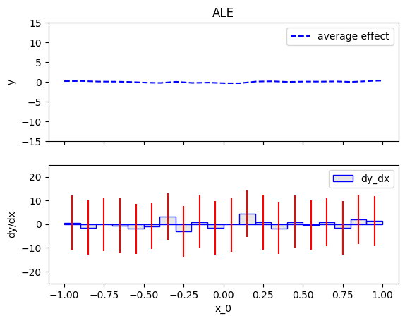
ALE is defined as: $$ \hat{f}^{ALE}(x_s) = TODO $$
The heterogeneity is: $$ TODO $$
The std of the bin-effects is: $$ TODO $$
Notes
- The required parameters are
dataandmodel. The rest are optional.
Parameters:
| Name | Type | Description | Default |
|---|---|---|---|
data
|
ndarray
|
the design matrix
|
required |
model
|
callable
|
the black-box model. Must be a
|
required |
nof_instances
|
Union[int, str]
|
the number of instances to use for the explanation
|
10000
|
axis_limits
|
Optional[ndarray]
|
The limits of the feature effect plot along each axis
|
None
|
feature_names
|
Optional[List]
|
The names of the features
|
None
|
target_name
|
Optional[str]
|
The name of the target variable
|
None
|
Methods:
| Name | Description |
|---|---|
fit |
Fit the ALE plot. |
eval |
Evalueate the (RH)ALE feature effect of feature |
plot |
Plot the (RH)ALE feature effect of feature |
Source code in effector/global_effect_ale.py
256 257 258 259 260 261 262 263 264 265 266 267 268 269 270 271 272 273 274 275 276 277 278 279 280 281 282 283 284 285 286 287 288 289 290 291 292 293 294 295 296 297 298 299 300 301 302 303 304 305 306 307 308 309 310 311 312 313 314 315 316 317 318 319 320 321 322 323 324 325 326 327 328 | |
fit(features='all', binning_method='fixed', centering=True, points_for_centering=30)
Fit the ALE plot.
Parameters:
| Name | Type | Description | Default |
|---|---|---|---|
features
|
Union[int, str, list]
|
the features to fit. If set to "all", all the features will be fitted. |
'all'
|
binning_method
|
Union[str, Fixed]
|
|
'fixed'
|
centering
|
Union[bool, str]
|
whether to compute the normalization constant for centering the plot:
|
True
|
points_for_centering
|
int
|
the number of points to use for centering the plot. Default is 100. |
30
|
Source code in effector/global_effect_ale.py
364 365 366 367 368 369 370 371 372 373 374 375 376 377 378 379 380 381 382 383 384 385 386 387 388 389 390 391 392 393 394 395 396 397 | |
eval(feature, xs, heterogeneity=False, centering=True, **kwargs)
Evalueate the (RH)ALE feature effect of feature feature at points xs.
Notes
This is a common method inherited by both ALE and RHALE.
Parameters:
| Name | Type | Description | Default |
|---|---|---|---|
feature
|
int
|
index of feature of interest |
required |
xs
|
ndarray
|
the points along the s-th axis to evaluate the FE plot
- |
required |
heterogeneity
|
bool
|
whether to return heterogeneity:
|
False
|
centering
|
Union[bool, str]
|
whether to center the plot:
|
True
|
Returns:
the mean effect y, if heterogeneity=False (default) or a tuple (y, std) otherwise
Source code in effector/global_effect_ale.py
107 108 109 110 111 112 113 114 115 116 117 118 119 120 121 122 123 124 125 126 127 128 129 130 131 132 133 134 135 136 137 138 139 140 141 142 143 144 145 146 147 148 149 150 151 152 153 154 155 156 157 158 | |
plot(feature, heterogeneity=True, centering=True, scale_x=None, scale_y=None, show_avg_output=False, y_limits=None, dy_limits=None, show_only_aggregated=False, show_plot=True)
Plot the (RH)ALE feature effect of feature feature.
Notes
This is a common method inherited by both ALE and RHALE.
Parameters:
| Name | Type | Description | Default |
|---|---|---|---|
feature
|
int
|
the feature to plot |
required |
heterogeneity
|
bool
|
whether to plot the heterogeneity
|
True
|
centering
|
Union[bool, str]
|
whether to center the plot:
|
True
|
scale_x
|
Optional[dict]
|
None or Dict with keys ['std', 'mean']
|
None
|
scale_y
|
Optional[dict]
|
None or Dict with keys ['std', 'mean']
|
None
|
show_avg_output
|
bool
|
if True, the average output will be shown as a horizontal line. |
False
|
y_limits
|
Optional[List]
|
None or tuple, the limits of the y-axis
|
None
|
dy_limits
|
Optional[List]
|
None or tuple, the limits of the dy-axis
|
None
|
show_only_aggregated
|
bool
|
if True, only the main ale plot will be shown |
False
|
show_plot
|
bool
|
if True, the plot will be shown |
True
|
Source code in effector/global_effect_ale.py
160 161 162 163 164 165 166 167 168 169 170 171 172 173 174 175 176 177 178 179 180 181 182 183 184 185 186 187 188 189 190 191 192 193 194 195 196 197 198 199 200 201 202 203 204 205 206 207 208 209 210 211 212 213 214 215 216 217 218 219 220 221 222 223 224 225 226 227 228 229 230 231 232 233 234 235 236 237 238 239 240 241 242 243 244 245 246 247 248 249 250 | |
effector.global_effect_ale.RHALE(data, model, model_jac=None, nof_instances=10000, axis_limits=None, data_effect=None, feature_names=None, target_name=None)
Bases: ALEBase
Constructor for RHALE.
Definition
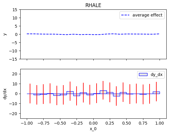
RHALE is defined as: $$ \hat{f}^{RHALE}(x_s) = TODO $$
The heterogeneity is: $$ TODO $$
The std of the bin-effects is: $$ TODO $$
Notes
The required parameters are data and model. The rest are optional.
Parameters:
| Name | Type | Description | Default |
|---|---|---|---|
data
|
ndarray
|
the design matrix
|
required |
model
|
callable
|
the black-box model. Must be a
|
required |
model_jac
|
Union[None, callable]
|
the Jacobian of the model. Must be a
|
None
|
nof_instances
|
Union[int, str]
|
the number of instances to use for the explanation
|
10000
|
axis_limits
|
Optional[ndarray]
|
The limits of the feature effect plot along each axis
|
None
|
data_effect
|
Optional[ndarray]
|
|
None
|
feature_names
|
Optional[list]
|
The names of the features
|
None
|
target_name
|
Optional[str]
|
The name of the target variable
|
None
|
Methods:
| Name | Description |
|---|---|
fit |
Fit the model. |
eval |
Evalueate the (RH)ALE feature effect of feature |
plot |
Plot the (RH)ALE feature effect of feature |
Source code in effector/global_effect_ale.py
401 402 403 404 405 406 407 408 409 410 411 412 413 414 415 416 417 418 419 420 421 422 423 424 425 426 427 428 429 430 431 432 433 434 435 436 437 438 439 440 441 442 443 444 445 446 447 448 449 450 451 452 453 454 455 456 457 458 459 460 461 462 463 464 465 466 467 468 469 470 471 472 473 474 475 476 477 478 479 480 481 482 | |
fit(features='all', binning_method='greedy', centering=True, points_for_centering=30)
Fit the model.
Parameters:
| Name | Type | Description | Default |
|---|---|---|---|
features
|
(int, str, list)
|
the features to fit.
|
'all'
|
binning_method
|
str
|
the binning method to use.
|
'greedy'
|
centering
|
Union[bool, str]
|
whether to compute the normalization constant for centering the plot:
|
True
|
points_for_centering
|
int
|
the number of points to use for centering the plot. Default is 100. |
30
|
Source code in effector/global_effect_ale.py
521 522 523 524 525 526 527 528 529 530 531 532 533 534 535 536 537 538 539 540 541 542 543 544 545 546 547 548 549 550 551 552 553 554 555 556 557 558 559 560 561 | |
eval(feature, xs, heterogeneity=False, centering=True, **kwargs)
Evalueate the (RH)ALE feature effect of feature feature at points xs.
Notes
This is a common method inherited by both ALE and RHALE.
Parameters:
| Name | Type | Description | Default |
|---|---|---|---|
feature
|
int
|
index of feature of interest |
required |
xs
|
ndarray
|
the points along the s-th axis to evaluate the FE plot
- |
required |
heterogeneity
|
bool
|
whether to return heterogeneity:
|
False
|
centering
|
Union[bool, str]
|
whether to center the plot:
|
True
|
Returns:
the mean effect y, if heterogeneity=False (default) or a tuple (y, std) otherwise
Source code in effector/global_effect_ale.py
107 108 109 110 111 112 113 114 115 116 117 118 119 120 121 122 123 124 125 126 127 128 129 130 131 132 133 134 135 136 137 138 139 140 141 142 143 144 145 146 147 148 149 150 151 152 153 154 155 156 157 158 | |
plot(feature, heterogeneity=True, centering=True, scale_x=None, scale_y=None, show_avg_output=False, y_limits=None, dy_limits=None, show_only_aggregated=False, show_plot=True)
Plot the (RH)ALE feature effect of feature feature.
Notes
This is a common method inherited by both ALE and RHALE.
Parameters:
| Name | Type | Description | Default |
|---|---|---|---|
feature
|
int
|
the feature to plot |
required |
heterogeneity
|
bool
|
whether to plot the heterogeneity
|
True
|
centering
|
Union[bool, str]
|
whether to center the plot:
|
True
|
scale_x
|
Optional[dict]
|
None or Dict with keys ['std', 'mean']
|
None
|
scale_y
|
Optional[dict]
|
None or Dict with keys ['std', 'mean']
|
None
|
show_avg_output
|
bool
|
if True, the average output will be shown as a horizontal line. |
False
|
y_limits
|
Optional[List]
|
None or tuple, the limits of the y-axis
|
None
|
dy_limits
|
Optional[List]
|
None or tuple, the limits of the dy-axis
|
None
|
show_only_aggregated
|
bool
|
if True, only the main ale plot will be shown |
False
|
show_plot
|
bool
|
if True, the plot will be shown |
True
|
Source code in effector/global_effect_ale.py
160 161 162 163 164 165 166 167 168 169 170 171 172 173 174 175 176 177 178 179 180 181 182 183 184 185 186 187 188 189 190 191 192 193 194 195 196 197 198 199 200 201 202 203 204 205 206 207 208 209 210 211 212 213 214 215 216 217 218 219 220 221 222 223 224 225 226 227 228 229 230 231 232 233 234 235 236 237 238 239 240 241 242 243 244 245 246 247 248 249 250 | |
effector.global_effect_pdp.PDP(data, model, axis_limits=None, nof_instances=10000, feature_names=None, target_name=None)
Bases: PDPBase
Constructor of the PDP class.
Definition
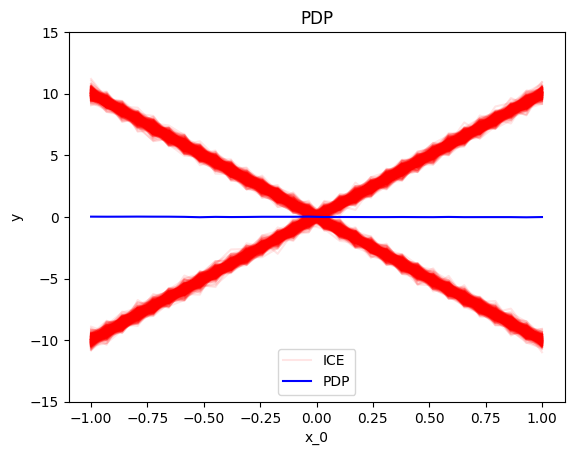
PDP: $$ PDP(x_s) = {1 \over N} \sum_{i=1}^N f(x_s, \mathbf{x}_c^i) $$
centered-PDP: $$ PDP_c(x_s) = PDP(x_s) - c, \quad c = {1 \over M} \sum_{j=1}^M PDP(x_s^j) $$
ICE: $$ ICE^i(x_s) = f(x_s, \mathbf{x}_c^i), \quad i=1, \dots, N $$
centered-ICE: $$ ICE_c^i(x_s) = ICE^i(x_s) - c_i, \quad c_i = {1 \over M} \sum_{j=1}^M ICE^i(x_s^j) $$
heterogeneity function: $$ h(x_s) = {1 \over N} \sum_{i=1}^N ( ICE_c^i(x_s) - PDP_c(x_s) )^2 $$
The heterogeneity value is: $$ \mathcal{H}(x_s) = {1 \over M} \sum_{j=1}^M h(x_s^j), $$ where \(x_s^j\) are an equally spaced grid of points in \([x_s^{\min}, x_s^{\max}]\).
Notes
The required parameters are data and model. The rest are optional.
Parameters:
| Name | Type | Description | Default |
|---|---|---|---|
data
|
ndarray
|
the design matrix
|
required |
model
|
Callable
|
the black-box model. Must be a
|
required |
axis_limits
|
Optional[ndarray]
|
The limits of the feature effect plot along each axis
|
None
|
nof_instances
|
Union[int, str]
|
maximum number of instances to be used
|
10000
|
feature_names
|
Optional[List]
|
The names of the features
|
None
|
target_name
|
Optional[str]
|
The name of the target variable
|
None
|
Methods:
| Name | Description |
|---|---|
fit |
Fit the Feature effect to the data. |
eval |
Evaluate the effect of the s-th feature at positions |
plot |
Plot the feature effect. |
Source code in effector/global_effect_pdp.py
243 244 245 246 247 248 249 250 251 252 253 254 255 256 257 258 259 260 261 262 263 264 265 266 267 268 269 270 271 272 273 274 275 276 277 278 279 280 281 282 283 284 285 286 287 288 289 290 291 292 293 294 295 296 297 298 299 300 301 302 303 304 305 306 307 308 309 310 311 312 313 314 315 316 317 318 319 320 321 322 323 324 325 326 327 328 329 | |
fit(features='all', centering=False, points_for_centering=30, use_vectorized=True)
Fit the Feature effect to the data.
Notes
You can use .eval or .plot without calling .fit explicitly.
The only thing that .fit does is to compute the normalization constant for centering the PDP and ICE plots.
This will be automatically done when calling eval or plot, so there is no need to call fit explicitly.
Parameters:
| Name | Type | Description | Default |
|---|---|---|---|
features
|
Union[int, str, list]
|
the features to fit. - If set to "all", all the features will be fitted. |
'all'
|
centering
|
Union[bool, str]
|
whether to center the plot:
|
False
|
points_for_centering
|
int
|
number of linspaced points along the feature axis used for centering. |
30
|
use_vectorized
|
bool
|
whether to use vectorized operations for the PDP and ICE curves |
True
|
Source code in effector/global_effect_pdp.py
68 69 70 71 72 73 74 75 76 77 78 79 80 81 82 83 84 85 86 87 88 89 90 91 92 93 94 95 96 97 98 99 100 101 102 103 104 105 106 107 108 | |
eval(feature, xs, heterogeneity=False, centering=False, return_all=False, use_vectorized=True)
Evaluate the effect of the s-th feature at positions xs.
Parameters:
| Name | Type | Description | Default |
|---|---|---|---|
feature
|
int
|
index of feature of interest |
required |
xs
|
ndarray
|
the points along the s-th axis to evaluate the FE plot
|
required |
heterogeneity
|
bool
|
whether to return the heterogeneity measures.
|
False
|
centering
|
Union[bool, str]
|
whether to center the PDP
|
False
|
return_all
|
bool
|
whether to return PDP and ICE plots evaluated at
|
False
|
use_vectorized
|
bool
|
whether to use the vectorized version of the computation |
True
|
Returns:
| Type | Description |
|---|---|
Union[ndarray, Tuple[ndarray, ndarray]]
|
the mean effect |
Source code in effector/global_effect_pdp.py
110 111 112 113 114 115 116 117 118 119 120 121 122 123 124 125 126 127 128 129 130 131 132 133 134 135 136 137 138 139 140 141 142 143 144 145 146 147 148 149 150 151 152 153 154 155 156 157 158 159 160 161 162 163 164 165 166 167 168 169 170 171 172 173 174 175 176 | |
plot(feature, heterogeneity='ice', centering=True, nof_points=30, scale_x=None, scale_y=None, nof_ice='all', show_avg_output=False, y_limits=None, use_vectorized=True, show_plot=True)
Plot the feature effect.
Parameters:
| Name | Type | Description | Default |
|---|---|---|---|
feature
|
int
|
the feature to plot |
required |
heterogeneity
|
Union[bool, str]
|
whether to plot the heterogeneity
|
'ice'
|
centering
|
Union[bool, str]
|
whether to center the plot
|
True
|
nof_points
|
int
|
the grid size for the PDP plot |
30
|
scale_x
|
Optional[dict]
|
None or Dict with keys ['std', 'mean']
|
None
|
scale_y
|
Optional[dict]
|
None or Dict with keys ['std', 'mean']
|
None
|
nof_ice
|
Union[int, str]
|
number of ICE plots to show on top of the SHAP curve |
'all'
|
show_avg_output
|
bool
|
whether to show the average output of the model |
False
|
y_limits
|
Optional[List]
|
None or tuple, the limits of the y-axis
|
None
|
use_vectorized
|
bool
|
whether to use the vectorized version of the PDP computation |
True
|
Source code in effector/global_effect_pdp.py
331 332 333 334 335 336 337 338 339 340 341 342 343 344 345 346 347 348 349 350 351 352 353 354 355 356 357 358 359 360 361 362 363 364 365 366 367 368 369 370 371 372 373 374 375 376 377 378 379 380 381 382 383 384 385 386 387 388 389 390 391 392 393 394 395 396 397 398 399 | |
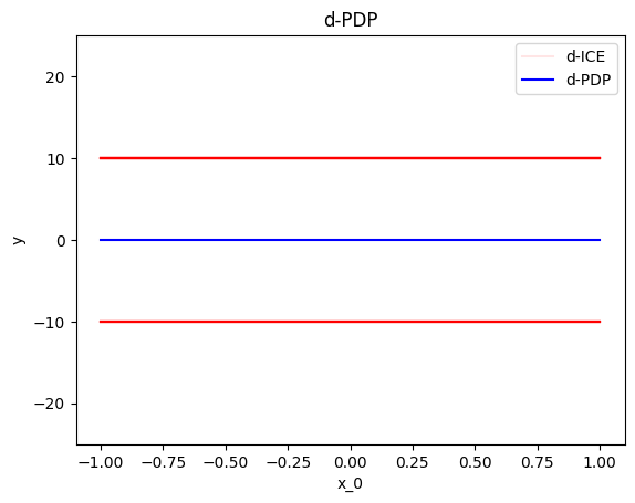
effector.global_effect_pdp.DerPDP(data, model, model_jac=None, axis_limits=None, nof_instances=10000, feature_names=None, target_name=None)
Bases: PDPBase
Constructor of the DerivativePDP class.
Definition
d-PDP: $$ dPDP(x_s) = {1 \over N} \sum_{i=1}^N {\partial f \over \partial x_s}(x_s, \mathbf{x}_c^i) $$
centered-PDP: $$ dPDP_c(x_s) = dPDP(x_s) - c, \quad c = {1 \over M} \sum_{j=1}^M dPDP(x_s^j) $$
ICE: $$ dICE^i(x_s) = {\partial f \over \partial x_s}(x_s, \mathbf{x}_c^i), \quad i=1, \dots, N $$
centered-ICE: $$ dICE_c^i(x_s) = dICE^i(x_s) - c_i, \quad c_i = {1 \over M} \sum_{j=1}^M dICE^i(x_s^j) $$
heterogeneity function: $$ h(x_s) = {1 \over N} \sum_{i=1}^N ( dICE_c^i(x_s) - dPDP_c(x_s) )^2 $$
The heterogeneity value is: $$ \mathcal{H}(x_s) = {1 \over M} \sum_{j=1}^M h(x_s^j), $$ where \(x_s^j\) are an equally spaced grid of points in \([x_s^{\min}, x_s^{\max}]\).
Notes
- The required parameters are
dataandmodel. The rest are optional. - The
model_jacis the Jacobian of the model. IfNone, the Jacobian will be computed numerically.
Parameters:
| Name | Type | Description | Default |
|---|---|---|---|
data
|
ndarray
|
the design matrix
|
required |
model
|
Callable
|
the black-box model. Must be a
|
required |
model_jac
|
Optional[Callable]
|
the black-box model Jacobian. Must be a
|
None
|
axis_limits
|
Optional[ndarray]
|
The limits of the feature effect plot along each axis
|
None
|
nof_instances
|
Union[int, str]
|
maximum number of instances to be used for PDP.
|
10000
|
feature_names
|
Optional[List]
|
The names of the features
|
None
|
target_name
|
Optional[str]
|
The name of the target variable
|
None
|
Methods:
| Name | Description |
|---|---|
fit |
Fit the Feature effect to the data. |
eval |
Evaluate the effect of the s-th feature at positions |
plot |
Plot the feature effect. |
Source code in effector/global_effect_pdp.py
403 404 405 406 407 408 409 410 411 412 413 414 415 416 417 418 419 420 421 422 423 424 425 426 427 428 429 430 431 432 433 434 435 436 437 438 439 440 441 442 443 444 445 446 447 448 449 450 451 452 453 454 455 456 457 458 459 460 461 462 463 464 465 466 467 468 469 470 471 472 473 474 475 476 477 478 479 480 481 482 483 484 485 486 487 488 489 490 491 492 493 494 495 496 | |
fit(features='all', centering=False, points_for_centering=30, use_vectorized=True)
Fit the Feature effect to the data.
Notes
You can use .eval or .plot without calling .fit explicitly.
The only thing that .fit does is to compute the normalization constant for centering the PDP and ICE plots.
This will be automatically done when calling eval or plot, so there is no need to call fit explicitly.
Parameters:
| Name | Type | Description | Default |
|---|---|---|---|
features
|
Union[int, str, list]
|
the features to fit. - If set to "all", all the features will be fitted. |
'all'
|
centering
|
Union[bool, str]
|
whether to center the plot:
|
False
|
points_for_centering
|
int
|
number of linspaced points along the feature axis used for centering. |
30
|
use_vectorized
|
bool
|
whether to use vectorized operations for the PDP and ICE curves |
True
|
Source code in effector/global_effect_pdp.py
68 69 70 71 72 73 74 75 76 77 78 79 80 81 82 83 84 85 86 87 88 89 90 91 92 93 94 95 96 97 98 99 100 101 102 103 104 105 106 107 108 | |
eval(feature, xs, heterogeneity=False, centering=False, return_all=False, use_vectorized=True)
Evaluate the effect of the s-th feature at positions xs.
Parameters:
| Name | Type | Description | Default |
|---|---|---|---|
feature
|
int
|
index of feature of interest |
required |
xs
|
ndarray
|
the points along the s-th axis to evaluate the FE plot
|
required |
heterogeneity
|
bool
|
whether to return the heterogeneity measures.
|
False
|
centering
|
Union[bool, str]
|
whether to center the PDP
|
False
|
return_all
|
bool
|
whether to return PDP and ICE plots evaluated at
|
False
|
use_vectorized
|
bool
|
whether to use the vectorized version of the computation |
True
|
Returns:
| Type | Description |
|---|---|
Union[ndarray, Tuple[ndarray, ndarray]]
|
the mean effect |
Source code in effector/global_effect_pdp.py
110 111 112 113 114 115 116 117 118 119 120 121 122 123 124 125 126 127 128 129 130 131 132 133 134 135 136 137 138 139 140 141 142 143 144 145 146 147 148 149 150 151 152 153 154 155 156 157 158 159 160 161 162 163 164 165 166 167 168 169 170 171 172 173 174 175 176 | |
plot(feature, heterogeneity='ice', centering=False, nof_points=30, scale_x=None, scale_y=None, nof_ice=100, show_avg_output=False, dy_limits=None, use_vectorized=True, show_plot=True)
Plot the feature effect.
Parameters:
| Name | Type | Description | Default |
|---|---|---|---|
feature
|
int
|
the feature to plot |
required |
heterogeneity
|
Union[bool, str]
|
whether to plot the heterogeneity
|
'ice'
|
centering
|
Union[bool, str]
|
whether to center the plot
|
False
|
nof_points
|
int
|
the grid size for the PDP plot |
30
|
scale_x
|
Optional[dict]
|
None or Dict with keys ['std', 'mean']
|
None
|
scale_y
|
Optional[dict]
|
None or Dict with keys ['std', 'mean']
|
None
|
nof_ice
|
Union[int, str]
|
number of ICE plots to show on top of the SHAP curve |
100
|
show_avg_output
|
bool
|
whether to show the average output of the model |
False
|
dy_limits
|
Optional[List]
|
None or tuple, the limits of the y-axis for the derivative PDP
|
None
|
use_vectorized
|
bool
|
whether to use the vectorized version of the PDP computation |
True
|
show_plot
|
bool
|
whether to show the plot |
True
|
Source code in effector/global_effect_pdp.py
498 499 500 501 502 503 504 505 506 507 508 509 510 511 512 513 514 515 516 517 518 519 520 521 522 523 524 525 526 527 528 529 530 531 532 533 534 535 536 537 538 539 540 541 542 543 544 545 546 547 548 549 550 551 552 553 554 555 556 557 558 559 560 561 562 563 564 565 566 567 568 | |
effector.global_effect_shap.ShapDP(data, model, axis_limits=None, nof_instances=1000, feature_names=None, target_name=None, shap_values=None, backend='shap')
Bases: GlobalEffectBase
Constructor of the ShapDP class.
Definition
The value of a coalition of \(S\) features is estimated as: $$ \hat{v}(S) = {1 \over N} \sum_{i=1}^N [f(\mathbf{x}_S \cup \mathbf{x}_C^i) - f(\mathbf{x}^i) ] $$ \(\hat{v}(S)\) quantifies the contribution when the features in \(S\) are set to \(\mathbf{x}_S\). For all instances, we compute two outputs:
- \(f(\mathbf{x}_S \cup \mathbf{x}_C^i)\) is the output of the model when the features in \(S\) are set to \(\mathbf{x}_S\) and the rest of the features are left as they are
- \(f(\mathbf{x}^i)\) is the output of the model when the instance is left as is The average difference (over all instances) between these two outputs is the value of the coalition \(S\).
The contribution of a feature \(j\) added to a coalition \(S\) is estimated as: $$ \hat{\Delta}_{S, j} = \hat{v}(S \cup {j}) - \hat{v}(S) $$
The SHAP value of a feature \(j\) with value \(x_j\) is the average contribution of feature \(j\) across all possible coalitions with a weight \(w_{S, j}\):
where \(w_{S, j}\) assures that the contribution of feature \(j\) is the same for all coalitions of the same size. For example, there are \(D-1\) ways for \(x_j\) to enter a coalition of \(|S| = 1\) feature, so \(w_{S, j} = {1 \over D (D-1)}\) for each of them. In contrast, there is only one way for \(x_j\) to enter a coaltion of \(|S|=0\) (to be the first specified feature), so \(w_{S, j} = {1 \over D}\).
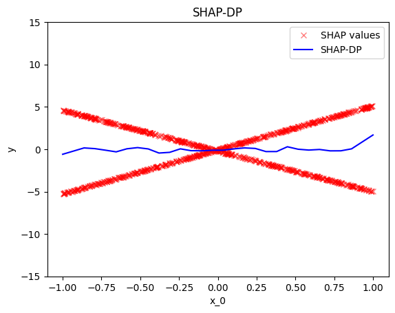
The SHAP Dependence Plot (SHAP-DP) is a spline \(\hat{f}^{SDP}_j(x_j)\) fit to the dataset \(\{(x_j^i, \hat{\phi}_j(x_j^i))\}_{i=1}^N\) using the UnivariateSpline function from scipy.interpolate.
Notes
- The required parameters are
dataandmodel. The rest are optional. - SHAP values are computed using either the
shappackage (backend="shap") or theshapiqpackage (backend="shapiq"). - SHAP values are centered by default, i.e., the average SHAP value is subtracted from the SHAP values.
- More details on the SHAP values can be found in the original paper and in the book Interpreting Machine Learning Models with SHAP
Parameters:
| Name | Type | Description | Default |
|---|---|---|---|
data
|
ndarray
|
the design matrix
|
required |
model
|
Callable
|
the black-box model. Must be a
|
required |
axis_limits
|
Optional[ndarray]
|
The limits of the feature effect plot along each axis
|
None
|
nof_instances
|
Union[int, str]
|
maximum number of instances to be used for SHAP estimation.
|
1000
|
avg_output
|
The average output of the model.
|
required | |
feature_names
|
Optional[List[str]]
|
The names of the features
|
None
|
target_name
|
Optional[str]
|
The name of the target variable
|
None
|
shap_values
|
Optional[ndarray]
|
The SHAP values of the model
|
None
|
backend
|
str
|
Package to compute SHAP values
|
'shap'
|
Notes
SHAP values are expensive to compute.
To speed up the computation consider using a subset of the dataset.
The nof_instances parameter controls the number of instances used for computing the SHAP values.
The default value is 1_000 instances, which is a good trade-off between speed and accuracy.
Methods:
| Name | Description |
|---|---|
fit |
Fit the SHAP Dependence Plot to the data. |
eval |
Evaluate the effect of the s-th feature at positions |
plot |
Plot the SHAP Dependence Plot (SDP) of the s-th feature. |
Source code in effector/global_effect_shap.py
15 16 17 18 19 20 21 22 23 24 25 26 27 28 29 30 31 32 33 34 35 36 37 38 39 40 41 42 43 44 45 46 47 48 49 50 51 52 53 54 55 56 57 58 59 60 61 62 63 64 65 66 67 68 69 70 71 72 73 74 75 76 77 78 79 80 81 82 83 84 85 86 87 88 89 90 91 92 93 94 95 96 97 98 99 100 101 102 103 104 105 106 107 108 109 110 111 112 113 114 115 116 117 118 119 120 121 122 123 124 125 126 127 | |
fit(features='all', centering=True, points_for_centering=30, binning_method='greedy', budget=512, shap_explainer_kwargs=None, shap_explanation_kwargs=None)
Fit the SHAP Dependence Plot to the data.
Notes
The SHAP Dependence Plot (SDP) \(\hat{f}^{SDP}_j(x_j)\) is a spline fit to
the dataset \(\{(x_j^i, \hat{\phi}_j(x_j^i))\}_{i=1}^N\)
using the UnivariateSpline function from scipy.interpolate.
The SHAP standard deviation, \(\hat{\sigma}^{SDP}_j(x_j)\), is a spline fit to the absolute value of the residuals, i.e., to the dataset \(\{(x_j^i, |\hat{\phi}_j(x_j^i) - \hat{f}^{SDP}_j(x_j^i)|)\}_{i=1}^N\), using the UnivariateSpline function from scipy.interpolate.
Parameters:
| Name | Type | Description | Default |
|---|---|---|---|
features
|
Union[int, str, List]
|
the features to fit. - If set to "all", all the features will be fitted. |
'all'
|
centering
|
Union[bool, str]
|
|
True
|
points_for_centering
|
Union[int, str]
|
number of linspaced points along the feature axis used for centering.
|
30
|
binning_method
|
Union[str, Greedy, Fixed]
|
the binning method to be used for fitting a piecewise linear function to the SHAP values.
|
'greedy'
|
budget
|
int
|
Budget to use for the approximation. Defaults to 512. - Increasing the budget improves the approximation at the cost of slower computation. - Decrease the budget for faster computation at the cost of approximation error. |
512
|
shap_explainer_kwargs
|
Optional[dict]
|
the keyword arguments to be passed to the Code behind the sceneCheck the code that is running behind the scene before customizing |
None
|
shap_explanation_kwargs
|
Optional[dict]
|
the keyword arguments to be passed to the Code behind the sceneCheck the code that is running behind the scene before customizing |
None
|
Source code in effector/global_effect_shap.py
225 226 227 228 229 230 231 232 233 234 235 236 237 238 239 240 241 242 243 244 245 246 247 248 249 250 251 252 253 254 255 256 257 258 259 260 261 262 263 264 265 266 267 268 269 270 271 272 273 274 275 276 277 278 279 280 281 282 283 284 285 286 287 288 289 290 291 292 293 294 295 296 297 298 299 300 301 302 303 304 305 306 307 308 309 310 311 312 313 314 315 316 317 318 319 320 321 322 323 324 325 326 327 328 329 330 331 332 333 334 335 336 337 338 339 340 341 342 343 344 345 346 347 348 349 350 351 352 353 354 355 356 357 358 359 360 361 362 363 364 365 366 367 368 369 370 | |
eval(feature, xs, heterogeneity=True, centering=True)
Evaluate the effect of the s-th feature at positions xs.
Parameters:
| Name | Type | Description | Default |
|---|---|---|---|
feature
|
int
|
index of feature of interest |
required |
xs
|
ndarray
|
the points along the s-th axis to evaluate the FE plot
|
required |
heterogeneity
|
bool
|
whether to return the heterogeneity measures.
|
True
|
centering
|
Union[bool, str]
|
whether to center the plot
|
True
|
Returns:
| Type | Description |
|---|---|
Union[ndarray, Tuple[ndarray, ndarray]]
|
the mean effect |
Source code in effector/global_effect_shap.py
372 373 374 375 376 377 378 379 380 381 382 383 384 385 386 387 388 389 390 391 392 393 394 395 396 397 398 399 400 401 402 403 404 405 406 407 408 409 410 411 412 413 414 415 416 417 418 | |
plot(feature, heterogeneity='shap_values', centering=True, nof_points=30, scale_x=None, scale_y=None, nof_shap_values='all', show_avg_output=False, y_limits=None, only_shap_values=False, show_plot=True)
Plot the SHAP Dependence Plot (SDP) of the s-th feature.
Parameters:
| Name | Type | Description | Default |
|---|---|---|---|
feature
|
int
|
index of the plotted feature |
required |
heterogeneity
|
Union[bool, str]
|
whether to output the heterogeneity of the SHAP values
|
'shap_values'
|
centering
|
Union[bool, str]
|
whether to center the SDP
|
True
|
nof_points
|
int
|
number of points to evaluate the SDP plot |
30
|
scale_x
|
Optional[dict]
|
dictionary with keys "mean" and "std" for scaling the x-axis |
None
|
scale_y
|
Optional[dict]
|
dictionary with keys "mean" and "std" for scaling the y-axis |
None
|
nof_shap_values
|
Union[int, str]
|
number of shap values to show on top of the SHAP curve |
'all'
|
show_avg_output
|
bool
|
whether to show the average output of the model |
False
|
y_limits
|
Optional[List]
|
limits of the y-axis |
None
|
only_shap_values
|
bool
|
whether to plot only the shap values |
False
|
show_plot
|
bool
|
whether to show the plot |
True
|
Source code in effector/global_effect_shap.py
420 421 422 423 424 425 426 427 428 429 430 431 432 433 434 435 436 437 438 439 440 441 442 443 444 445 446 447 448 449 450 451 452 453 454 455 456 457 458 459 460 461 462 463 464 465 466 467 468 469 470 471 472 473 474 475 476 477 478 479 480 481 482 483 484 485 486 487 488 489 490 491 492 493 494 495 496 497 498 499 500 501 502 503 504 505 506 507 508 509 510 511 512 513 514 | |