Bike-Sharing Dataset
- Author: givasile
- Runtime: ~6 min
- Description: The canonical effector workflow on a real dataset — scope →
triage → look → find regions → triage with arrows — explaining a neural
network trained on hourly bike-rental counts, with per-method deep dives
(PDP, RHALE, SHAP-DP) on the
hourfeature. - 📄 The whole notebook in one page: PDP report
This notebook analyzes the Capital Bikeshare system's rental data from 2011-2012. We'll explore how various factors influence bike rental patterns using advanced machine learning techniques. The Bike-Sharing Dataset contains: - 17,379 hourly records - 14 features including temporal and weather information - Target variable: hourly bike rental count
import effector
import numpy as np
import tensorflow as tf
from tensorflow import keras
import random

np.random.seed(42)
tf.random.set_seed(42)
random.seed(42)
WARNING: All log messages before absl::InitializeLog() is called are written to STDERR
I0000 00:00:1784068177.633870   24871 cpu_feature_guard.cc:227] This TensorFlow binary is optimized to use available CPU instructions in performance-critical operations.
To enable the following instructions: AVX2 FMA, in other operations, rebuild TensorFlow with the appropriate compiler flags.
Preprocess the data
from ucimlrepo import fetch_ucirepo
bike_sharing_dataset = fetch_ucirepo(id=275)
X = bike_sharing_dataset.data.features
y = bike_sharing_dataset.data.targets
X = X.drop(["dteday", "atemp"], axis=1)
print("Design matrix shape: {}".format(X.shape))
print("---------------------------------")
for i, col_name in enumerate(X.columns):
    print("x_{} {:15}, unique: {:4d}, Mean: {:6.2f}, Std: {:6.2f}, Min: {:6.2f}, Max: {:6.2f}".format(i, col_name, len(X[col_name].unique()), X[col_name].mean(), X[col_name].std(), X[col_name].min(), X[col_name].max()))

print("\nTarget shape: {}".format(y.shape))
print("---------------------------------")
for col_name in y.columns:
    print("Target: {:15}, unique: {:4d}, Mean: {:6.2f}, Std: {:6.2f}, Min: {:6.2f}, Max: {:6.2f}".format(col_name, len(y[col_name].unique()), y[col_name].mean(), y[col_name].std(), y[col_name].min(), y[col_name].max()))
Design matrix shape: (17379, 11)
---------------------------------
x_0 season         , unique:    4, Mean:   2.50, Std:   1.11, Min:   1.00, Max:   4.00
x_1 yr             , unique:    2, Mean:   0.50, Std:   0.50, Min:   0.00, Max:   1.00
x_2 mnth           , unique:   12, Mean:   6.54, Std:   3.44, Min:   1.00, Max:  12.00
x_3 hr             , unique:   24, Mean:  11.55, Std:   6.91, Min:   0.00, Max:  23.00
x_4 holiday        , unique:    2, Mean:   0.03, Std:   0.17, Min:   0.00, Max:   1.00
x_5 weekday        , unique:    7, Mean:   3.00, Std:   2.01, Min:   0.00, Max:   6.00
x_6 workingday     , unique:    2, Mean:   0.68, Std:   0.47, Min:   0.00, Max:   1.00
x_7 weathersit     , unique:    4, Mean:   1.43, Std:   0.64, Min:   1.00, Max:   4.00
x_8 temp           , unique:   50, Mean:   0.50, Std:   0.19, Min:   0.02, Max:   1.00
x_9 hum            , unique:   89, Mean:   0.63, Std:   0.19, Min:   0.00, Max:   1.00
x_10 windspeed      , unique:   30, Mean:   0.19, Std:   0.12, Min:   0.00, Max:   0.85

Target shape: (17379, 1)
---------------------------------
Target: cnt            , unique:  869, Mean: 189.46, Std: 181.39, Min:   1.00, Max: 977.00
def preprocess(X, y):
    # Standarize X
    X_df = X
    x_mean = X_df.mean()
    x_std = X_df.std()
    X_df = (X_df - X_df.mean()) / X_df.std()

    # Standarize Y
    Y_df = y
    y_mean = Y_df.mean()
    y_std = Y_df.std()
    Y_df = (Y_df - Y_df.mean()) / Y_df.std()
    return X_df, Y_df, x_mean, x_std, y_mean, y_std

# shuffle and standarize all features
X_df, Y_df, x_mean, x_std, y_mean, y_std = preprocess(X, y)
def split(X_df, Y_df):
    # shuffle indices
    indices = X_df.index.tolist()
    np.random.shuffle(indices)

    # data split
    train_size = int(0.8 * len(X_df))

    X_train = X_df.iloc[indices[:train_size]]
    Y_train = Y_df.iloc[indices[:train_size]]
    X_test = X_df.iloc[indices[train_size:]]
    Y_test = Y_df.iloc[indices[train_size:]]

    return X_train, Y_train, X_test, Y_test

# train/test split
X_train, Y_train, X_test, Y_test = split(X_df, Y_df)
Fit a Neural Network
# Train - Evaluate - Explain a neural network
model = keras.Sequential([
    keras.layers.Dense(1024, activation="relu"),
    keras.layers.Dense(512, activation="relu"),
    keras.layers.Dense(256, activation="relu"),
    keras.layers.Dense(1)
])

optimizer = keras.optimizers.Adam(learning_rate=0.001)
model.compile(optimizer=optimizer, loss="mse", metrics=["mae", keras.metrics.RootMeanSquaredError()])
model.fit(X_train, Y_train, batch_size=512, epochs=20, verbose=0)
print("train [mse, mae, rmse]:", [round(v, 3) for v in model.evaluate(X_train, Y_train, verbose=0)])
print("test  [mse, mae, rmse]:", [round(v, 3) for v in model.evaluate(X_test, Y_test, verbose=0)])
train [mse, mae, rmse]: [0.047, 0.155, 0.216]


test  [mse, mae, rmse]: [0.068, 0.176, 0.26]
We train a deep fully-connected Neural Network with 3 hidden layers for \(20\) epochs. The model achieves a root mean squared error on the test of about \(0.24\) units, that corresponds to approximately \(0.26 * 181 = 47\) counts.
Explain
effector needs a numpy-in / numpy-out callable. For sklearn or torch models, effector.adapters builds this wrapper for you (adapters.from_sklearn, adapters.from_torch); keras wrappers stay hand-written, like model_forward below.
def model_jac(x):
    x_tensor = tf.convert_to_tensor(x, dtype=tf.float32)
    with tf.GradientTape() as t:
        t.watch(x_tensor)
        pred = model(x_tensor)
        grads = t.gradient(pred, x_tensor)
    return grads.numpy()

def model_forward(x):
    return model(x).numpy().squeeze()

# the handshake: probe the wrapper before building engines
effector.adapters.check(model_forward, X_train.to_numpy())
scale_y = {"mean": y_mean.iloc[0], "std": y_std.iloc[0]}
scale_x_list =[{"mean": x_mean.iloc[i], "std": x_std.iloc[i]} for i in range(len(x_mean))]
scale_x = scale_x_list[3]
feature_names = X_df.columns.to_list()
target_name = "bike-rentals"
y_limits=[-200, 800]
dy_limits = [-300, 300]
feature_types = [
    "nominal",     # 0  season
    "nominal",     # 1  yr
    "ordinal",     # 2  mnth
    "ordinal",     # 3  hr
    "nominal",     # 4  holiday
    "nominal",     # 5  weekday
    "nominal",     # 6  workingday
    "ordinal",     # 7  weathersit
    "continuous",  # 8  temp
    "continuous",  # 9  hum
    "continuous",  # 10 windspeed
]
# level names, ascending by the observed (standardized) level values — the
# raw encodings are ordered, so the order survives standardization
category_names = [
    ["winter", "spring", "summer", "fall"],              # 0 season (1-4)
    ["2011", "2012"],                                    # 1 yr
    ["Jan", "Feb", "Mar", "Apr", "May", "Jun",
     "Jul", "Aug", "Sep", "Oct", "Nov", "Dec"],          # 2 mnth
    None,                                                # 3 hr (numeric ticks)
    ["no", "yes"],                                       # 4 holiday
    ["Sun", "Mon", "Tue", "Wed", "Thu", "Fri", "Sat"],   # 5 weekday
    ["no", "yes"],                                       # 6 workingday
    ["clear", "mist", "light rain/snow", "heavy rain"],  # 7 weathersit
    None, None, None,                                    # 8-10 temp/hum/windspeed
]
scale_x_list[8]["mean"] += 8
scale_x_list[8]["std"] *= 47

scale_x_list[9]["std"] *= 100
scale_x_list[10]["std"] *= 67

# the full schema: names, types, level names, and the inverse scaling —
# every report, rule, and tick renders in raw units and level names
schema = effector.Schema(
    feature_names=feature_names,
    feature_types=feature_types,
    category_names=category_names,
    scale_x_list=scale_x_list,
    scale_y=scale_y,
    target_name=target_name,
)
Survey all features: the triage plane
Instead of eyeballing every feature's plot one by one, effector.plot_triage surveys them in a single figure: importance to the right, heterogeneity up. The top-right corner — important and heterogeneous — is the to-do list: those are the features whose mean effect hides something and where find_regions should look. The horizontal hairline is the median-heterogeneity threshold, the same convention find_regions(features="heterogeneous") uses.
We scope the survey to the numerical features, where feature effect methods are most meaningful:
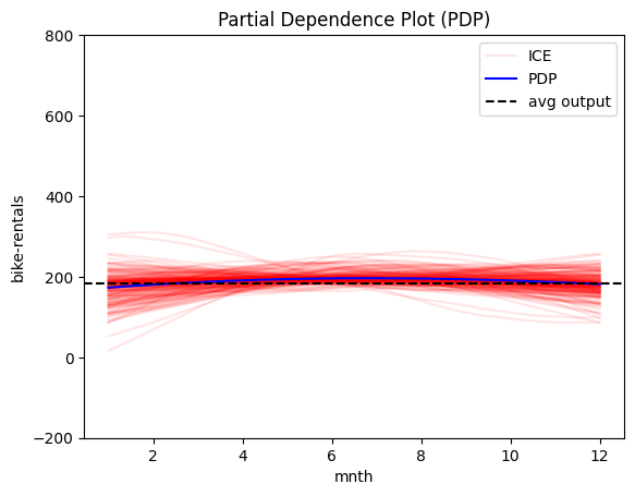
monthhrtemphumiditywindspeed
pdp = effector.PDP(data=X_train.to_numpy(), model=model_forward, schema=schema, nof_instances=2000)
pdp.fit(features=[2, 3, 8, 9, 10], centering=True)
effector.plot_triage(pdp, features=[2, 3, 8, 9, 10])
# the per-feature look, reusing the same fitted engine
for i in [2, 3, 8, 9, 10]:
    pdp.plot(feature=i, centering=True, scale_x=scale_x_list[i], scale_y=scale_y, show_avg_output=True, nof_ice=200, y_limits=y_limits)
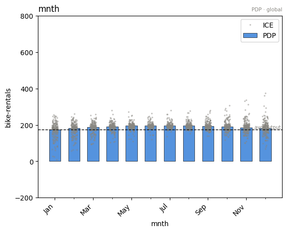
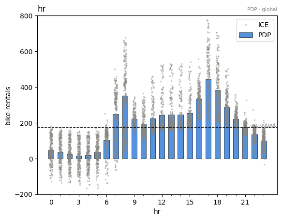
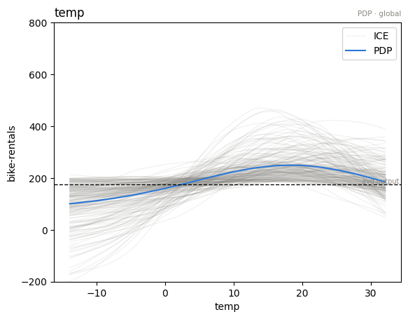
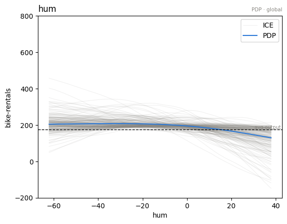
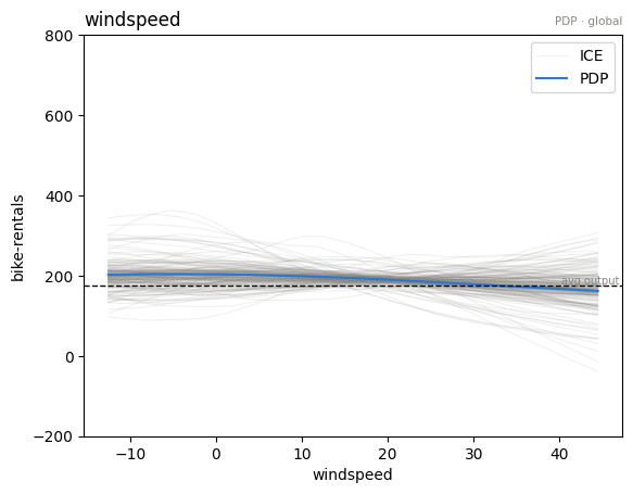
We observe that features: hour, temperature and humidity have an intersting structure. Out of them hour has by far the most influence on the output, so it makes sensce to focus on it further.
Feature hour
All global methods at a glance
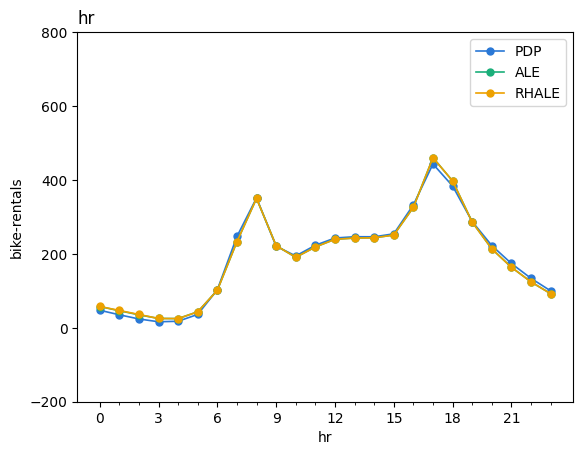
Before diving into each method separately, we can compare them in a single figure with the unified effector.FeatureEffect API. It holds the data/model/scaling once and overlays the (centered) mean effect of each method, so differences between methods are immediately visible. ShapDP can be added to the list too (it is slower, so it is opt-in).
fe = effector.FeatureEffect(
    X_train.to_numpy(),
    model_forward,
    model_jac=model_jac,
    schema=schema,
    nof_instances=2000,
)
fe.plot(
    feature=3,
    methods=["PDP", "ALE", "RHALE"],
    centering=True,
    scale_x=scale_x,
    scale_y=scale_y,
    y_limits=y_limits,
)
PDP - global
pdp = effector.PDP(data=X_train.to_numpy(), model=model_forward, schema=schema, nof_instances=5000)
pdp.plot(feature="hr", centering=True, scale_x=scale_x, scale_y=scale_y, show_avg_output=True, nof_ice=200)
Importance and one-click explanation
Beyond the per-feature effect curves, the fitted global effect exposes an importances()
vector (the dispersion of each feature's mean effect — the \(\mu\)-twin of heterogeneity), and
effector.explain(...) runs the whole pipeline once and returns a serializable Report.
# per-feature importance = dispersion of the mean effect (mu-twin of heterogeneity)
print("importances:", np.round(pdp.importances(), 3))

# one-click auto-explanation -> Report (serializable; self-contained HTML)
report = effector.explain(
    X_train.to_numpy(),
    model_forward,
    y=Y_train.to_numpy().squeeze(),
    method="pdp",
    schema=schema,
    nof_instances=2000,
)
report.show()

# the whole notebook, in one page: the report published with this example
from pathlib import Path
_out = Path("reports") / "01_bike_sharing_dataset"
_out.mkdir(parents=True, exist_ok=True)
report.to_html(_out / "report_pdp.html")
importances: [0.09  0.191 0.04  0.663 0.022 0.044 0.041 0.053 0.228 0.112 0.018]


[effector] global effects   (GAM)  -> 71.7% of the model's variance
           regional effects (CALM) -> 88.6%

  ════════════════════════════════════════════════════════════════════════
  PDP report  ·  target: bike-rentals
  ════════════════════════════════════════════════════════════════════════

  DATA & MODEL
  ────────────────────────────────────────────────────────────────────────
    instances     2,000
    features      11  ·  5 nominal · 3 ordinal · 3 continuous
    model output  mean 174 · std 177 · range [-48.9, 928]
    model R²      0.947  (on this subsample)

  EXPLAINED VARIANCE
  ────────────────────────────────────────────────────────────────────────
    step         split on                 solo     ΔR²      R²       heter
    ──────────────────────────────────────────────────────────────────────
    GAM          (all features global)       —       —   71.7%           —
  + hr           temp, workingday, yr   +15.5%  +15.5%   87.2% 0.48 → 0.29
  + hum          hr, temp, weathersit    +1.8%   +1.4%   88.6% 0.17 → 0.15
    ──────────────────────────────────────────────────────────────────────
    FINAL                                                88.6%

  REJECTED SPLITS                                            min gain 1.0%
  ────────────────────────────────────────────────────────────────────────
    feature      split on                 solo     ΔR²    reason
    ──────────────────────────────────────────────────────────────────────
  ✗ temp         hr, hum                 +1.7%   +0.9%    below threshold
  ✗ yr           hr, hum                 +1.5%   -0.1%    redundant
  ✗ workingday   hr, yr                  +4.9%   -4.3%    redundant

    ✗ redundant: it would explain variance on its own (see solo),
      but the accepted splits already account for it.

  FEATURES                                ranked, in the selected snapshot
  ────────────────────────────────────────────────────────────────────────
    feature        importance                          heter      #regions
    ──────────────────────────────────────────────────────────────────────
    hr                 0.7314  ██████████████████     0.2882             4
    temp               0.2281  ██████                 0.2668             1
    yr                 0.1878  █████                  0.2028             1
    hum                0.1020  ███                    0.1525             4
    ──────────────────────────────────────────────────────────────────────
    the features above carry 80% of the total importance mass


Feature 3 - Full partition tree:
🌳 Full Tree Structure:
───────────────────────
hr 🔹 [id: 0 | heter: 0.48 | inst: 2000 | w: 1.00]
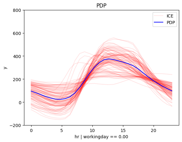
    workingday = no 🔹 [id: 1 | heter: 0.37 | inst: 614 | w: 0.31]
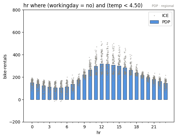
        temp < 4.50 🔹 [id: 2 | heter: 0.24 | inst: 248 | w: 0.12]
        temp ≥ 4.50 🔹 [id: 3 | heter: 0.32 | inst: 366 | w: 0.18]
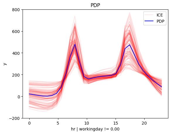
    workingday = yes 🔹 [id: 4 | heter: 0.34 | inst: 1386 | w: 0.69]
        yr = 2011 🔹 [id: 5 | heter: 0.25 | inst: 696 | w: 0.35]
        yr = 2012 🔹 [id: 6 | heter: 0.32 | inst: 690 | w: 0.34]
--------------------------------------------------
Feature 3 - Statistics per tree level:
🌳 Tree Summary:
─────────────────
Level 0🔹heter: 0.48
    Level 1🔹heter: 0.35 | 🔻0.13 (26.67%)
        Level 2🔹heter: 0.29 | 🔻0.06 (17.80%)


Feature 9 - Full partition tree:
🌳 Full Tree Structure:
───────────────────────
hum 🔹 [id: 0 | heter: 0.17 | inst: 2000 | w: 1.00]
    temp < 13.71 🔹 [id: 1 | heter: 0.15 | inst: 1338 | w: 0.67]
        weathersit = light rain/snow 🔹 [id: 2 | heter: 0.33 | inst: 146 | w: 0.07]
        weathersit ∈ {clear, mist, heavy rain} 🔹 [id: 3 | heter: 0.12 | inst: 1192 | w: 0.60]
    temp ≥ 13.71 🔹 [id: 4 | heter: 0.18 | inst: 662 | w: 0.33]
        hr = 17.00 🔹 [id: 5 | heter: 0.19 | inst: 33 | w: 0.02]
        hr ∈ {0.00, 1.00, 2.00, …} (23 levels) 🔹 [id: 6 | heter: 0.17 | inst: 629 | w: 0.31]
--------------------------------------------------
Feature 9 - Statistics per tree level:
🌳 Tree Summary:
─────────────────
Level 0🔹heter: 0.17
    Level 1🔹heter: 0.16 | 🔻0.01 (7.69%)
        Level 2🔹heter: 0.15 | 🔻0.01 (5.23%)


/home/givasile/github/packages/effector/effector/report.py:606: UserWarning: This figure includes Axes that are not compatible with tight_layout, so results might be incorrect.
  fig.tight_layout()
PDP - regional
pdp_reg = effector.PDP(data=X_train.to_numpy(), model=model_forward, schema=schema, nof_instances=5_000)
pdp_reg.fit("hr", centering=True)
part_pdp = pdp_reg.find_regions("hr", finder="best")
part_pdp.show(scale_x_list=scale_x_list)
Feature 3 - Full partition tree:
🌳 Full Tree Structure:
───────────────────────
hr 🔹 [id: 0 | heter: 0.48 | inst: 5000 | w: 1.00]
    workingday = no 🔹 [id: 1 | heter: 0.37 | inst: 1563 | w: 0.31]
        temp < 4.50 🔹 [id: 2 | heter: 0.24 | inst: 642 | w: 0.13]
        temp ≥ 4.50 🔹 [id: 3 | heter: 0.33 | inst: 921 | w: 0.18]
    workingday = yes 🔹 [id: 4 | heter: 0.34 | inst: 3437 | w: 0.69]
        yr = 2011 🔹 [id: 5 | heter: 0.25 | inst: 1762 | w: 0.35]
        yr = 2012 🔹 [id: 6 | heter: 0.32 | inst: 1675 | w: 0.34]
--------------------------------------------------
Feature 3 - Statistics per tree level:
🌳 Tree Summary:
─────────────────
Level 0🔹heter: 0.48
    Level 1🔹heter: 0.35 | 🔻0.13 (26.72%)
        Level 2🔹heter: 0.29 | 🔻0.06 (18.37%)
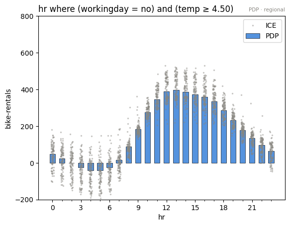
# plot the level-1 subregions (region idx == old node_idx)
for r in part_pdp:
    if r.level == 1:
        part_pdp.plot(r.idx, centering=True, scale_x_list=scale_x_list, scale_y=scale_y, y_limits=y_limits)
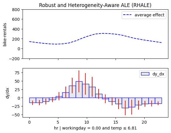
The same node, ad hoc: any verb takes rule= — here node 1's rule straight from the partition.
pdp_reg.plot("hr", rule=part_pdp[1].rule, centering=True, scale_x=scale_x, scale_y=scale_y, y_limits=y_limits)
# and the level-2 subregions, where the tree splits further
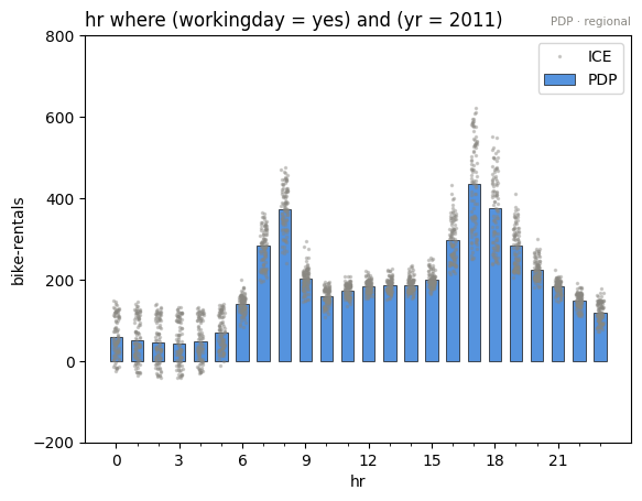
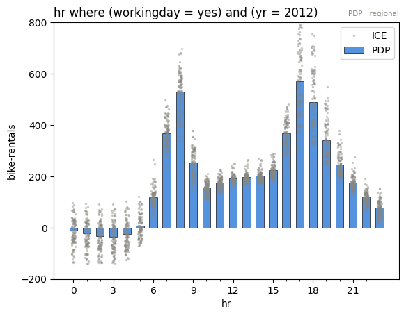
for r in part_pdp:
    if r.level == 2:
        part_pdp.plot(r.idx, centering=True, scale_x_list=scale_x_list, scale_y=scale_y, y_limits=y_limits)
Triage, after: the before/after arrows
The same triage plane, revisited with partitions=: for every partitioned feature an arrow runs from its global point to each leaf point (the leaf's importance/heterogeneity under its rule). Leaves of a good partition move right and down — more decisive, less heterogeneous. Here, splitting hr on workingday does exactly that.
effector.plot_triage(pdp_reg, features=[2, 3, 8, 9, 10], partitions={"hr": part_pdp})
RHALE - global
rhale = effector.RHALE(data=X_train.to_numpy(), model=model_forward, model_jac=model_jac, schema=schema)
rhale.plot(feature="hr", heterogeneity="std", centering=True, scale_x=scale_x, scale_y=scale_y, show_avg_output=True)
PDP vs RHALE on one axis
effector.compare overlays engines you already hold — method disagreement is information. The curves are always centered, so only shape differences remain.
effector.compare(pdp, rhale, feature="hr", scale_x=scale_x_list[3], scale_y=scale_y, y_limits=y_limits)
RHALE - regional
rhale_reg = effector.RHALE(data=X_train.to_numpy(), model=model_forward, model_jac=model_jac, schema=schema)
rhale_reg.fit("hr", centering=True)
part_rhale = rhale_reg.find_regions("hr", finder="best")
part_rhale.show(scale_x_list=scale_x_list)
Feature 3 - Full partition tree:
🌳 Full Tree Structure:
───────────────────────
hr 🔹 [id: 0 | heter: 2.24 | inst: 10000 | w: 1.00]
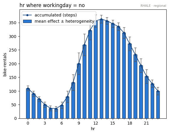
    workingday = no 🔹 [id: 1 | heter: 0.80 | inst: 3148 | w: 0.31]
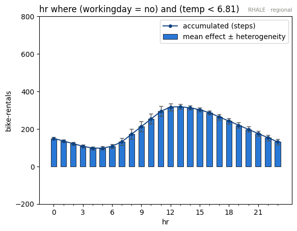
        temp < 6.81 🔹 [id: 2 | heter: 0.62 | inst: 1577 | w: 0.16]
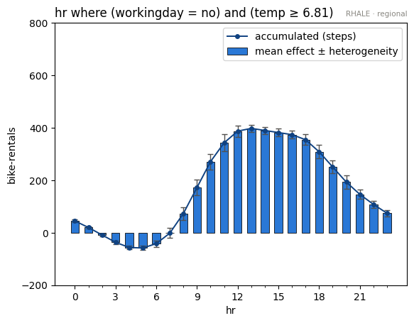
        temp ≥ 6.81 🔹 [id: 3 | heter: 0.70 | inst: 1571 | w: 0.16]
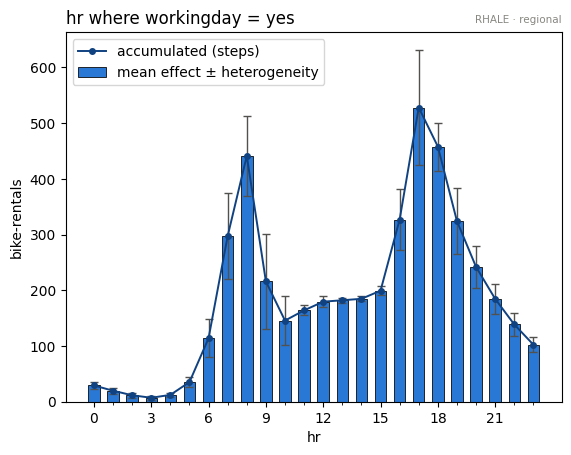
    workingday = yes 🔹 [id: 4 | heter: 1.63 | inst: 6852 | w: 0.69]
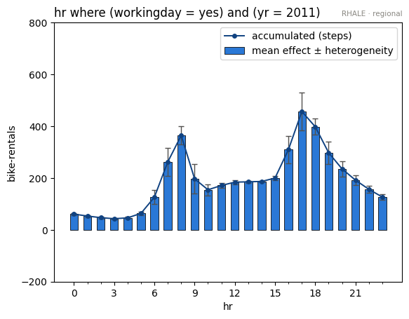
        yr = 2011 🔹 [id: 5 | heter: 1.15 | inst: 3463 | w: 0.35]
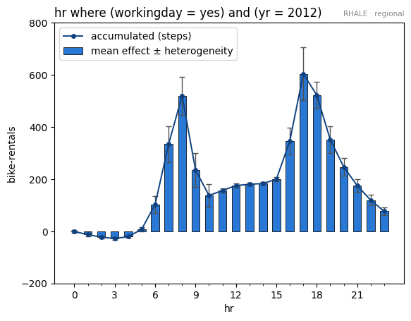
        yr = 2012 🔹 [id: 6 | heter: 1.52 | inst: 3389 | w: 0.34]
--------------------------------------------------
Feature 3 - Statistics per tree level:
🌳 Tree Summary:
─────────────────
Level 0🔹heter: 2.24
    Level 1🔹heter: 1.37 | 🔻0.87 (38.77%)
        Level 2🔹heter: 1.12 | 🔻0.25 (18.48%)
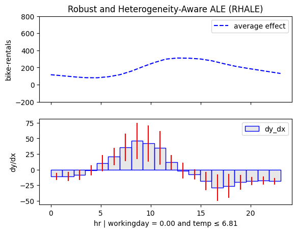
for r in part_rhale:
    if r.level == 1:
        part_rhale.plot(r.idx, centering=True, scale_x_list=scale_x_list, scale_y=scale_y)
for r in part_rhale:
    if r.level == 2:
        part_rhale.plot(r.idx, centering=True, scale_x_list=scale_x_list, scale_y=scale_y, y_limits=y_limits)
SHAPDP - global
shap_dp = effector.ShapDP(data=X_train.to_numpy(), model=model_forward, schema=schema, nof_instances=500)
shap_dp.plot(feature="hr", centering=True, scale_x=scale_x, scale_y=scale_y, show_avg_output=True)
SHAPDP - regional
shap_dp_reg = effector.ShapDP(data=X_train.to_numpy(), model=model_forward, schema=schema, nof_instances=500)
shap_dp_reg.fit("hr", centering=True)
part_shap = shap_dp_reg.find_regions("hr", finder="best")
part_shap.show(scale_x_list=scale_x_list)
Feature 3 - Full partition tree:
🌳 Full Tree Structure:
───────────────────────
hr 🔹 [id: 0 | heter: 0.23 | inst: 500 | w: 1.00]
    workingday = no 🔹 [id: 1 | heter: 0.13 | inst: 155 | w: 0.31]
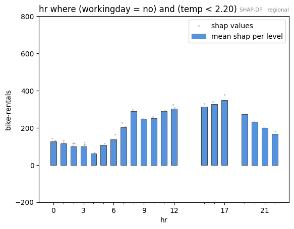
        temp < 2.20 🔹 [id: 2 | heter: 0.09 | inst: 59 | w: 0.12]
        temp ≥ 2.20 🔹 [id: 3 | heter: 0.11 | inst: 96 | w: 0.19]
    workingday = yes 🔹 [id: 4 | heter: 0.16 | inst: 345 | w: 0.69]
        yr = 2011 🔹 [id: 5 | heter: 0.11 | inst: 173 | w: 0.35]
        yr = 2012 🔹 [id: 6 | heter: 0.11 | inst: 172 | w: 0.34]
--------------------------------------------------
Feature 3 - Statistics per tree level:
🌳 Tree Summary:
─────────────────
Level 0🔹heter: 0.23
    Level 1🔹heter: 0.15 | 🔻0.08 (34.60%)
        Level 2🔹heter: 0.11 | 🔻0.04 (26.71%)
for r in part_shap:
    if r.level == 1:
        part_shap.plot(r.idx, centering=True, scale_x_list=scale_x_list, scale_y=scale_y)
for r in part_shap:
    if r.level == 2:
        part_shap.plot(r.idx, centering=True, scale_x_list=scale_x_list, scale_y=scale_y, y_limits=y_limits)
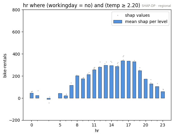
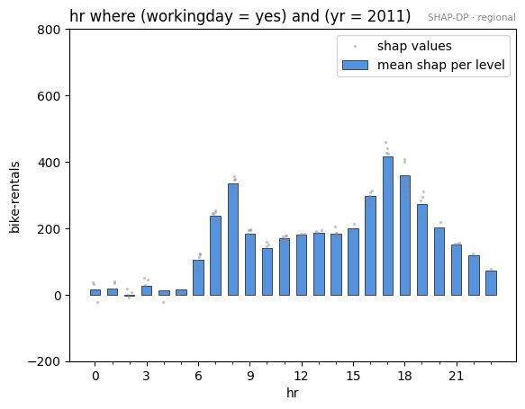
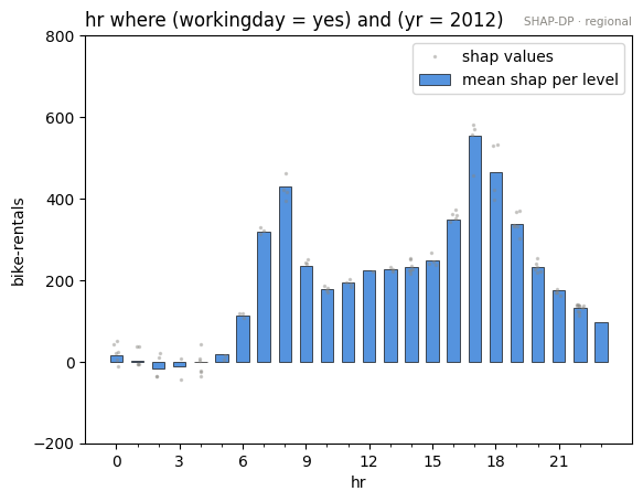
Conclusion
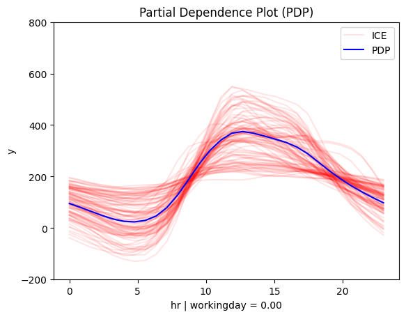
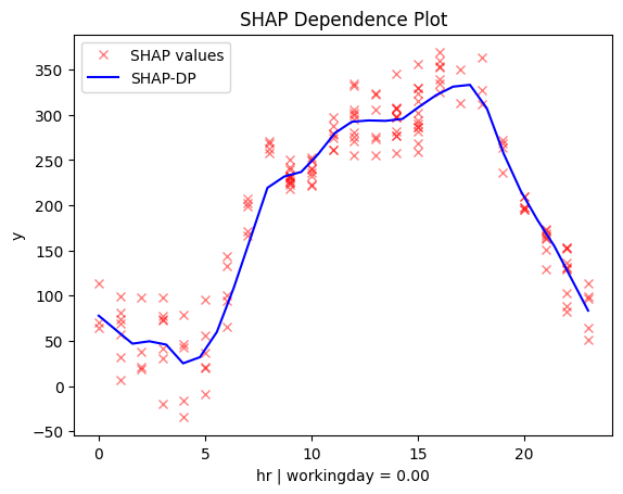
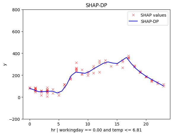
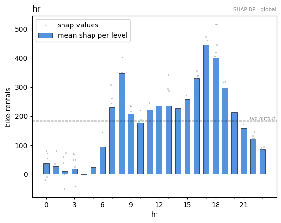
Global effect of hour All methods agree: hour has a strong influence on bike rentals, showing two clear peaks—around 8:00 and 17:00. This likely reflects commute times. But the exact shape of the effect varies between methods, hinting that local (regional) patterns could help explain these differences.
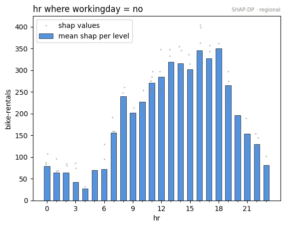
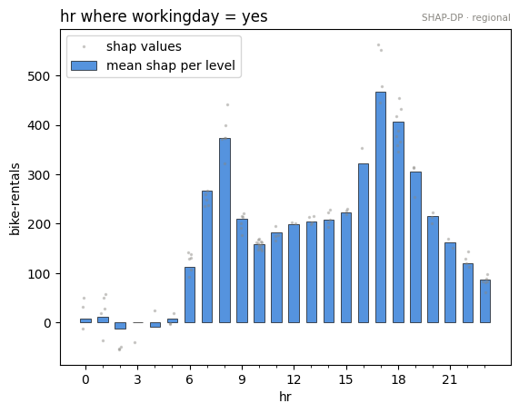
Regional effect of hour When we zoom in using regional methods, two patterns emerge:
- On working days, the effect follows the global trend, with peaks at 8:00 and 17:00—again, probably due to commuting.
- On non-working days, we see a single peak around 13:00, which makes sense if people are out enjoying leisure activities or sightseeing.
All methods agree up to this point.
Interactions Looking deeper, we see some interesting (but weaker) interactions. Most methods highlight either temperature or year (whether it’s the first or second year of data) as relevant.
For example, RHALE shows that on non-working days, the midday peak (12:00–14:00) becomes even stronger when the temperature is higher. That fits our intuition—people are more likely to rent bikes when it’s warm and sunny.
The workflow
This notebook is the canonical effector pipeline: (a) scope the features and hand the model over (adapters.check), (b) triage them on the importance × heterogeneity plane (plot_triage), (c) look at the effects that matter (plot), (d) partition the heterogeneous ones (find_regions + leaf plots), and (e) close the loop with the before/after arrows (plot_triage(..., partitions=...)). For the reasoning behind each step, see the mental-model page (../../quickstart/mental_model.md).
Cross-method sanity check
The one-liner effector.explain with every engine this notebook's model
supports. Everything must run end to end; the closing table puts the reads
side by side. Where methods disagree — ranking, accepted splits, R² — that is
a property of the data/model worth a closer look, not an error.
from pathlib import Path
_out = Path("reports") / "01_bike_sharing_dataset"
_out.mkdir(parents=True, exist_ok=True)

# === cross-method sweep: effector.explain on every applicable engine ======
sweep_reports = {}
for _m in ["pdp", "derpdp", "ale", "rhale", "shapdp"]:
    _kw = {"nof_instances": 300} if _m == "shapdp" else {}
    print(f"--- {_m} " + "-" * 50)
    sweep_reports[_m] = effector.explain(
        X_train.to_numpy(), model_forward, model_jac,
        y=Y_train.to_numpy().squeeze(), method=_m, schema=schema, **_kw
    )
    if _m != "pdp":  # the published report is the narrated one above
        sweep_reports[_m].to_html(_out / f"report_{_m}.html")

print()
print(f"{'method':<8} {'ranking (plotted)':<44} {'GAM R2':>8} {'final R2':>9}  splits")
for _m, _r in sweep_reports.items():
    _rank = " > ".join(fr.name for fr in _r.features)
    _ev = _r.explained_variance
    if _ev:
        _sp = "; ".join(f"{s['name']} on {s['on']}" for s in _ev["stages"]) or "none"
        print(f"{_m:<8} {_rank:<44} {_ev['gam_r2']:>7.1%} {_ev['regional_r2']:>8.1%}  {_sp}")
    else:
        print(f"{_m:<8} {_rank:<44} {'-':>7} {'-':>8}  (derivative scale: no variance ledger)")

print(f"\nreports stored in {_out}/")
--- pdp --------------------------------------------------


[effector] global effects   (GAM)  -> 71.3% of the model's variance
           regional effects (CALM) -> 88.7%
--- derpdp --------------------------------------------------


/home/givasile/github/packages/effector/effector/report.py:606: UserWarning: This figure includes Axes that are not compatible with tight_layout, so results might be incorrect.
  fig.tight_layout()


W0000 00:00:1784068630.950851   24871 cpu_allocator_impl.cc:82] Allocation of 4014080000 exceeds 10% of free system memory.


W0000 00:00:1784068631.815626   24871 cpu_allocator_impl.cc:82] Allocation of 4014080000 exceeds 10% of free system memory.


W0000 00:00:1784068632.990134   24871 cpu_allocator_impl.cc:82] Allocation of 4014080000 exceeds 10% of free system memory.


W0000 00:00:1784068641.638159   24871 cpu_allocator_impl.cc:82] Allocation of 4014080000 exceeds 10% of free system memory.


W0000 00:00:1784068648.413415   24871 cpu_allocator_impl.cc:82] Allocation of 4014080000 exceeds 10% of free system memory.


--- ale --------------------------------------------------


[effector] global effects   (GAM)  -> 71.0% of the model's variance
           regional effects (CALM) -> 88.8%


/home/givasile/github/packages/effector/effector/report.py:606: UserWarning: This figure includes Axes that are not compatible with tight_layout, so results might be incorrect.
  fig.tight_layout()


--- rhale --------------------------------------------------


[effector] global effects   (GAM)  -> 70.6% of the model's variance
           regional effects (CALM) -> 88.4%


/home/givasile/github/packages/effector/effector/report.py:606: UserWarning: This figure includes Axes that are not compatible with tight_layout, so results might be incorrect.
  fig.tight_layout()


--- shapdp --------------------------------------------------


[effector] global effects   (GAM)  -> 75.0% of the model's variance
           regional effects (CALM) -> 88.4%


/home/givasile/github/packages/effector/effector/report.py:606: UserWarning: This figure includes Axes that are not compatible with tight_layout, so results might be incorrect.
  fig.tight_layout()


method   ranking (plotted)                              GAM R2  final R2  splits
pdp      hr > temp > yr > hum                           71.3%    88.7%  hr on temp, workingday, yr
derpdp   hr > temp > yr                                     -        -  (derivative scale: no variance ledger)
ale      hr > yr > temp > season > hum                  71.0%    88.8%  hr on temp, workingday, yr
rhale    hr > yr > temp > season > hum                  70.6%    88.4%  hr on temp, workingday, yr
shapdp   hr > temp > yr > hum > season                  75.0%    88.4%  hr on temp, workingday, yr; temp on hum

reports stored in reports/01_bike_sharing_dataset/