Medical Costs — one interaction, two claimants
- Author: givasile
- Runtime: ~1 min
- Description: the variance ledger on the classic Medical Cost Personal
dataset —
global effects reproduce 84% of a gradient-boosted model, one split
(
bmi, conditioned onsmokerandage) recovers the rest, and the decision sequence shows whysmoker— the most important feature in the model — is redundant as a split:bmiandsmokerare two claimants of the same interaction pot. - 📄 The whole notebook in one page: PDP report
The dataset: 1,338 insurance policyholders with 6 features (age, sex,
bmi, children, smoker, region); the target is the yearly medical
charges billed to each person, in USD. It is the textbook example of a
conditional interaction: bmi matters a lot — but only for smokers.
import effector
import numpy as np

np.random.seed(21)
Load the data
effector.datasets.MedicalCosts fetches the CSV, encodes the categorical
columns to integer codes (recording the level names), and does a seeded 80/20
split. Everything stays in natural units — so the partition rules below
read directly as bmi < 30, smoker = yes.
data = effector.datasets.MedicalCosts()

print(f"X_train: {data.x_train.shape}, X_test: {data.x_test.shape}")
print("-" * 62)
for i, name in enumerate(data.feature_names):
    col = data.x_train[:, i]
    cats = data.category_names[i]
    levels = f" levels: {cats}" if cats else ""
    print(f"x_{i} {name:10s} [{data.feature_types[i]:10s}] "
          f"min: {col.min():7.1f}, max: {col.max():7.1f}{levels}")
print("-" * 62)
print(f"target: {data.target_name} ($/year), "
      f"mean: {data.y_train.mean():.0f}, std: {data.y_train.std():.0f}")
X_train: (1070, 6), X_test: (268, 6)
--------------------------------------------------------------
x_0 age        [continuous] min:    18.0, max:    64.0
x_1 sex        [nominal   ] min:     0.0, max:     1.0 levels: ['female', 'male']
x_2 bmi        [continuous] min:    16.8, max:    53.1
x_3 children   [ordinal   ] min:     0.0, max:     5.0
x_4 smoker     [nominal   ] min:     0.0, max:     1.0 levels: ['no', 'yes']
x_5 region     [nominal   ] min:     0.0, max:     3.0 levels: ['northeast', 'northwest', 'southeast', 'southwest']
--------------------------------------------------------------
target: charges ($/year), mean: 13438, std: 12295
Fit a model
A HistGradientBoostingRegressor — fast, deterministic, and strong on this
dataset.
from sklearn.ensemble import HistGradientBoostingRegressor
from sklearn.metrics import r2_score

model = HistGradientBoostingRegressor(random_state=21).fit(data.x_train, data.y_train)
print(f"train R^2 = {r2_score(data.y_train, model.predict(data.x_train)):.3f}")
print(f"test  R^2 = {r2_score(data.y_test, model.predict(data.x_test)):.3f}")
train R^2 = 0.945
test  R^2 = 0.813
Explain
effector needs a numpy-in / numpy-out callable; for sklearn regressors
effector.adapters.from_sklearn builds (and validates) the wrapper. The
schema comes straight off the loader.
model_forward = effector.adapters.from_sklearn(model)
effector.adapters.check(model_forward, data.x_train)

schema = effector.Schema(
    feature_names=data.feature_names,
    feature_types=data.feature_types,
    category_names=data.category_names,
    target_name=data.target_name,
)
The one-click report
effector.explain runs the whole pipeline — fit, rank, search regions,
select the splits worth keeping — and its headline is the variance
ledger: how much of the model's variance the global (GAM-style) curves
reproduce, and how much each accepted split adds.
from pathlib import Path
_out = Path("reports") / "05_medical_costs"
_out.mkdir(parents=True, exist_ok=True)

report = effector.explain(
    data=data.x_train,
    model=model_forward,
    y=data.y_train,
    schema=schema,
    method="pdp",
    nof_instances=5000,
)
report.show()
report.to_html(_out / "report_pdp.html")  # open in browser
[effector] global effects   (GAM)  -> 84.4% of the model's variance
           regional effects (CALM) -> 96.6%

  ════════════════════════════════════════════════════════════════════════
  PDP report  ·  target: charges
  ════════════════════════════════════════════════════════════════════════

  DATA & MODEL
  ────────────────────────────────────────────────────────────────────────
    instances     1,070
    features      6  ·  2 continuous · 3 nominal · 1 ordinal
    model output  mean 1.34e+04 · std 1.17e+04 · range [-100, 5.23e+04]
    model R²      0.945  (on this subsample)

  EXPLAINED VARIANCE
  ────────────────────────────────────────────────────────────────────────
    step         split on                 solo     ΔR²      R²       heter
    ──────────────────────────────────────────────────────────────────────
    GAM          (all features global)       —       —   84.4%           —
  + bmi          age, smoker            +12.1%  +12.1%   96.6% 4497 → 1229
    ──────────────────────────────────────────────────────────────────────
    FINAL                                                96.6%

  REJECTED SPLITS                                            min gain 1.0%
  ────────────────────────────────────────────────────────────────────────
    feature      split on                 solo     ΔR²    reason
    ──────────────────────────────────────────────────────────────────────
  ✗ smoker       bmi                    +11.1%  -11.5%    redundant
  ✗ age          bmi, children, smok…    +0.1%   +0.4%    below threshold

    ✗ redundant: it would explain variance on its own (see solo),
      but the accepted splits already account for it.

  FEATURES                                ranked, in the selected snapshot
  ────────────────────────────────────────────────────────────────────────
    feature        importance                          heter      #regions
    ──────────────────────────────────────────────────────────────────────
    smoker          9741.7124  ██████████████████  4202.7570             1
    age             3665.6089  ███████             1547.5959             1
    bmi             2669.0218  █████               1229.4831             4
    ──────────────────────────────────────────────────────────────────────
    the features above carry 91% of the total importance mass


Feature 2 - Full partition tree:
🌳 Full Tree Structure:
───────────────────────
bmi 🔹 [id: 0 | heter: 4497.23 | inst: 1070 | w: 1.00]
    smoker = no 🔹 [id: 1 | heter: 1439.97 | inst: 841 | w: 0.79]
        age < 43.30 🔹 [id: 2 | heter: 1162.94 | inst: 485 | w: 0.45]
        age ≥ 43.30 🔹 [id: 3 | heter: 1423.27 | inst: 356 | w: 0.33]
    smoker = yes 🔹 [id: 4 | heter: 1224.35 | inst: 229 | w: 0.21]
        age < 41.00 🔹 [id: 5 | heter: 1111.57 | inst: 125 | w: 0.12]
        age ≥ 41.00 🔹 [id: 6 | heter: 1018.18 | inst: 104 | w: 0.10]
--------------------------------------------------
Feature 2 - Statistics per tree level:
🌳 Tree Summary:
─────────────────
Level 0🔹heter: 4497.23
    Level 1🔹heter: 1393.82 | 🔻3103.41 (69.01%)
        Level 2🔹heter: 1229.48 | 🔻164.34 (11.79%)


/home/givasile/github/packages/effector/effector/report.py:606: UserWarning: This figure includes Axes that are not compatible with tight_layout, so results might be incorrect.
  fig.tight_layout()
The decision sequence, step by step
select_regions is the verb behind the ledger: greedy forward selection over
the candidate partitions, re-measuring every remaining split's marginal gain
each round. It returns a CalmSequence — the chain of snapshots from the
pure GAM to the final CALM.
pdp = effector.PDP(data.x_train, model_forward, schema=schema, nof_instances=5000)
chain = pdp.select_regions()
chain.show()
  EXPLAINED VARIANCE
  ────────────────────────────────────────────────────────────────────────
    step         split on                 solo     ΔR²      R²       heter
    ──────────────────────────────────────────────────────────────────────
    GAM          (all features global)       —       —   84.4%           —
  + bmi          age, smoker            +12.1%  +12.1%   96.6% 4497 → 1229
    ──────────────────────────────────────────────────────────────────────
    FINAL                                                96.6%

  REJECTED SPLITS                                            min gain 1.0%
  ────────────────────────────────────────────────────────────────────────
    feature      split on                 solo     ΔR²    reason
    ──────────────────────────────────────────────────────────────────────
  ✗ age          bmi, children, smok…    +0.1%   +0.4%    below threshold
  ✗ smoker       bmi                    +11.1%  -11.5%    redundant

    ✗ redundant: it would explain variance on its own (see solo),
      but the accepted splits already account for it.
Two claimants, one pot
The interesting line in the ledger is the rejected one. Solo — measured directly on top of the GAM — the two candidate splits are nearly equivalent:
- split
bmionsmoker/age: +12.1 pts - split
smokeronbmi: +11.1 pts
But they describe the same interaction. The interaction variance between
bmi and smoker is one pot, and both splits are claims on it. The greedy
sequence hands the pot to the best claimant (bmi | smoker, age); measured
after that, the smoker split's marginal gain collapses to ~0 and it is
skipped as redundant.
Redundant means already accounted for — not unimportant. smoker remains
by far the strongest main effect in the model (its importance dwarfs
everything else in the report's ranked table); it just has no additional
interaction variance to convert once the bmi split is in.
# the two-claimants signature, in numbers: solo gain vs sequential marginal
for s in chain.skipped:
    print(f"{s['name']:8s} solo: {s['solo_delta_r2']:+6.1%} | "
          f"after the accepted splits: {s['delta_r2']:+6.1%} [{s['reason']}]")
age      solo:  +0.1% | after the accepted splits:  +0.4% [below_threshold]
smoker   solo: +11.1% | after the accepted splits: -11.5% [redundant]
Look at the regions
The partition that won the pot, in feature units.
parts = pdp.find_regions("bmi", finder="best")
parts.show()
Feature 2 - Full partition tree:
🌳 Full Tree Structure:
───────────────────────
bmi 🔹 [id: 0 | heter: 4497.23 | inst: 1070 | w: 1.00]
    smoker = no 🔹 [id: 1 | heter: 1439.97 | inst: 841 | w: 0.79]
        age < 43.30 🔹 [id: 2 | heter: 1162.94 | inst: 485 | w: 0.45]
        age ≥ 43.30 🔹 [id: 3 | heter: 1423.27 | inst: 356 | w: 0.33]
    smoker = yes 🔹 [id: 4 | heter: 1224.35 | inst: 229 | w: 0.21]
        age < 41.00 🔹 [id: 5 | heter: 1111.57 | inst: 125 | w: 0.12]
        age ≥ 41.00 🔹 [id: 6 | heter: 1018.18 | inst: 104 | w: 0.10]
--------------------------------------------------
Feature 2 - Statistics per tree level:
🌳 Tree Summary:
─────────────────
Level 0🔹heter: 4497.23
    Level 1🔹heter: 1393.82 | 🔻3103.41 (69.01%)
        Level 2🔹heter: 1229.48 | 🔻164.34 (11.79%)
for r in parts:
    if r.level == 1:
        parts.plot(r.idx, centering=True)
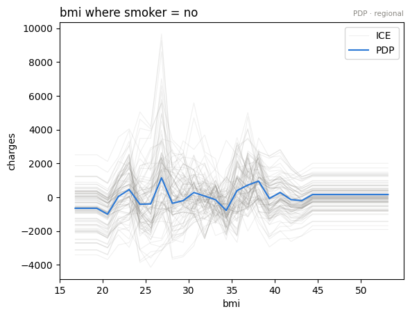
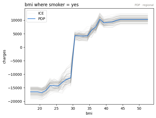
The split reads exactly like the domain story: for non-smokers, the
bmi curve is essentially flat — body mass barely moves the predicted
charges. For smokers, charges jump by roughly $15–20k past
bmi ≈ 30 (the clinical obesity threshold). The global bmi curve is the
average of these two regimes and represents neither.
effector.plot_triage(pdp, partitions={"bmi": parts})
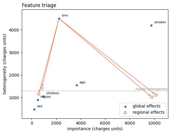
On the triage plane the arrows close the loop: the bmi leaves move
right and down — more decisive, less heterogeneous — which is what a good
partition does.
Conclusion
- Global curves explain 84% of this model; they are a fair summary of
age,children,region— and ofsmoker's big main effect. - The missing 12 pts live in one conditional interaction:
bmi × smoker. One split recovers it (→ 97%). - The decision sequence is the honest bookkeeping:
smoker | bmiis redundant as a split precisely becausebmi | smokeralready cashed the same pot. A report that showed both solo numbers would double-count.
Cross-method sanity check
The one-liner effector.explain with every engine this notebook's model
supports. A gradient-boosted tree is piecewise-constant, so derivative-scale
methods (RHALE, DerPDP) have no meaningful gradients to work with and are out
of scope here; PDP, ALE and SHAP-DP cover the output-scale reads. Where
methods disagree — ranking, accepted splits, R² — that is a property of the
data/model worth a closer look, not an error.
from pathlib import Path
_out = Path("reports") / "05_medical_costs"
_out.mkdir(parents=True, exist_ok=True)

# === cross-method sweep: effector.explain on every applicable engine ======
sweep_reports = {}
for _m in ["pdp", "ale", "shapdp"]:
    _kw = {"nof_instances": 300} if _m == "shapdp" else {"nof_instances": 5000}
    print(f"--- {_m} " + "-" * 50)
    sweep_reports[_m] = effector.explain(
        data.x_train, model_forward, y=data.y_train, method=_m, schema=schema, **_kw
    )
    if _m != "pdp":  # the published report is the narrated one above
        sweep_reports[_m].to_html(_out / f"report_{_m}.html")

print()
print(f"{'method':<8} {'ranking (plotted)':<52} {'GAM R2':>8} {'final R2':>9}  splits")
for _m, _r in sweep_reports.items():
    _rank = " > ".join(fr.name for fr in _r.features)
    _ev = _r.explained_variance
    _sp = "; ".join(f"{s['name']} on {s['on']}" for s in _ev["stages"]) or "none"
    print(f"{_m:<8} {_rank:<52} {_ev['gam_r2']:>7.1%} {_ev['regional_r2']:>8.1%}  {_sp}")

print(f"\nreports stored in {_out}/")
--- pdp --------------------------------------------------


[effector] global effects   (GAM)  -> 84.4% of the model's variance
           regional effects (CALM) -> 96.6%
--- ale --------------------------------------------------


[effector] global effects   (GAM)  -> 84.0% of the model's variance
           regional effects (CALM) -> 96.1%


/home/givasile/github/packages/effector/effector/report.py:606: UserWarning: This figure includes Axes that are not compatible with tight_layout, so results might be incorrect.
  fig.tight_layout()


--- shapdp --------------------------------------------------


[effector] global effects   (GAM)  -> 83.8% of the model's variance
           regional effects (CALM) -> 96.7%


/home/givasile/github/packages/effector/effector/report.py:606: UserWarning: This figure includes Axes that are not compatible with tight_layout, so results might be incorrect.
  fig.tight_layout()


method   ranking (plotted)                                      GAM R2  final R2  splits
pdp      smoker > age > bmi                                     84.4%    96.6%  bmi on age, smoker
ale      smoker > age > bmi                                     84.0%    96.1%  bmi on age, smoker
shapdp   smoker > age > bmi                                     83.8%    96.7%  bmi on children, smoker; smoker on bmi

reports stored in reports/05_medical_costs/