Adult Census Income — explaining a classifier's probability
- Author: givasile
- Runtime: ~5 min
- Description: the variance ledger on a classifier — effector explains
the predicted probability
P(income > 50K)of a gradient-boosted model on the Adult census dataset (UCI id 2). The probability surface turns out to be deeply interactive: global curves reproduce 72%, and it takes four splits — conditioned onage,marital-status,capital-gainandeducation-num— to reach 86%. - 📄 The whole notebook in one page: PDP report
The dataset: 45,222 census records (after dropping rows with missing
values); the target is whether yearly income exceeds $50K. The model is a
HistGradientBoostingClassifier; effector sees only its
predict_proba(...)[:, 1] — a numpy → numpy function like any other.
import effector
import numpy as np

np.random.seed(21)
Load the data
effector.datasets.AdultIncome drops fnlwgt (a sampling weight) and
education (duplicated by education-num), encodes the categorical columns
to integer codes with the level names recorded, and buckets levels rarer
than 50 rows into "Other" — a level that rare can vanish from a train
split, leaving the schema promising a category the data never shows.
data = effector.datasets.AdultIncome()

print(f"X_train: {data.x_train.shape}, X_test: {data.x_test.shape}")
print("-" * 66)
for i, name in enumerate(data.feature_names):
    cats = data.category_names[i]
    extra = f"{len(cats)} levels" if cats else "numeric"
    print(f"x_{i:<2} {name:16s} [{data.feature_types[i]:10s}] {extra}")
print("-" * 66)
print(f"target: {data.target_name}, base rate: {data.y_train.mean():.1%}")
X_train: (36177, 12), X_test: (9045, 12)
------------------------------------------------------------------
x_0  age              [continuous] numeric
x_1  workclass        [nominal   ] 7 levels
x_2  education-num    [ordinal   ] numeric
x_3  marital-status   [nominal   ] 7 levels
x_4  occupation       [nominal   ] 14 levels
x_5  relationship     [nominal   ] 6 levels
x_6  race             [nominal   ] 5 levels
x_7  sex              [nominal   ] 2 levels
x_8  capital-gain     [continuous] numeric
x_9  capital-loss     [continuous] numeric
x_10 hours-per-week   [continuous] numeric
x_11 native-country   [nominal   ] 25 levels
------------------------------------------------------------------
target: income>50K, base rate: 24.9%
Fit a classifier
from sklearn.ensemble import HistGradientBoostingClassifier
from sklearn.metrics import roc_auc_score

clf = HistGradientBoostingClassifier(random_state=21).fit(data.x_train, data.y_train)
print(f"test AUC = {roc_auc_score(data.y_test, clf.predict_proba(data.x_test)[:, 1]):.3f}")
test AUC = 0.925
Explain
Class labels are not a regression surface — effector explains a per-class
probability. effector.adapters.classifier_proba wraps
predict_proba(...)[:, class_] into the numpy → numpy callable every engine
expects. From here on, everything — curves, heterogeneity, the ledger — is
in probability units.
model_forward = effector.adapters.classifier_proba(clf, class_=1)
effector.adapters.check(model_forward, data.x_train)

schema = effector.Schema(
    feature_names=data.feature_names,
    feature_types=data.feature_types,
    category_names=data.category_names,
    target_name=data.target_name,
)
The one-click report
from pathlib import Path
_out = Path("reports") / "07_adult_income"
_out.mkdir(parents=True, exist_ok=True)

report = effector.explain(
    data=data.x_train,
    model=model_forward,
    y=data.y_train,
    schema=schema,
    method="pdp",
    nof_instances=5000,
)
report.show()
report.to_html(_out / "report_pdp.html")  # open in browser
[effector] global effects   (GAM)  -> 72.5% of the model's variance
           regional effects (CALM) -> 86.0%

  ════════════════════════════════════════════════════════════════════════
  PDP report  ·  target: income>50K
  ════════════════════════════════════════════════════════════════════════

  DATA & MODEL
  ────────────────────────────────────────────────────────────────────────
    instances     5,000
    features      12  ·  4 continuous · 7 nominal · 1 ordinal
    model output  mean 0.249 · std 0.309 · range [0.000225, 0.999]
    model accuracy0.879  (on this subsample)

  EXPLAINED VARIANCE
  ────────────────────────────────────────────────────────────────────────
    step         split on                 solo     ΔR²      R²       heter
    ──────────────────────────────────────────────────────────────────────
    GAM          (all features global)       —       —   72.5%           —
  + education-numage, capital-gain, …    +7.9%   +7.9%   80.4% 0.07 → 0.04
  + capital-gain age, education-num,…    +6.4%   +2.9%   83.2% 0.25 → 0.16
  + capital-loss age, capital-gain, …    +5.5%   +1.7%   85.0% 0.11 → 0.08
  + hours-per-weeage, capital-gain, …    +5.5%   +1.0%   86.0% 0.06 → 0.04
    ──────────────────────────────────────────────────────────────────────
    FINAL                                                86.0%

  REJECTED SPLITS                                            min gain 1.0%
  ────────────────────────────────────────────────────────────────────────
    feature      split on                 solo     ΔR²    reason
    ──────────────────────────────────────────────────────────────────────
  ✗ age          hours-per-week, mar…    +5.1%   +0.7%    below threshold
  ✗ relationship age, marital-status     +3.9%   +0.3%    below threshold

    ✗ redundant: it would explain variance on its own (see solo),
      but the accepted splits already account for it.

  FEATURES                                ranked, in the selected snapshot
  ────────────────────────────────────────────────────────────────────────
    feature        importance                          heter      #regions
    ──────────────────────────────────────────────────────────────────────
    capital-gain       0.1096  ██████████████████     0.1621             4
    age                0.0709  ████████████           0.0862             1
    education-num      0.0699  ███████████            0.0404             4
    capital-loss       0.0659  ███████████            0.0836             4
    relationship       0.0525  █████████              0.0561             1
    hours-per-week     0.0351  ██████                 0.0448             4
    ──────────────────────────────────────────────────────────────────────
    the features above carry 75% of the total importance mass


Feature 8 - Full partition tree:
🌳 Full Tree Structure:
───────────────────────
capital-gain 🔹 [id: 0 | heter: 0.25 | inst: 5000 | w: 1.00]
    marital-status = Married-civ-spouse 🔹 [id: 1 | heter: 0.23 | inst: 2319 | w: 0.46]
        education-num = 13.00 🔹 [id: 2 | heter: 0.17 | inst: 436 | w: 0.09]
        education-num ∈ {1.00, 2.00, 3.00, …} (15 levels) 🔹 [id: 3 | heter: 0.22 | inst: 1883 | w: 0.38]
    marital-status ∈ {Divorced, Married-spouse-absent, Never-married, …} (6 levels) 🔹 [id: 4 | heter: 0.21 | inst: 2681 | w: 0.54]
        age < 20.65 🔹 [id: 5 | heter: 0.08 | inst: 304 | w: 0.06]
        age ≥ 20.65 🔹 [id: 6 | heter: 0.12 | inst: 2377 | w: 0.48]
--------------------------------------------------
Feature 8 - Statistics per tree level:
🌳 Tree Summary:
─────────────────
Level 0🔹heter: 0.25
    Level 1🔹heter: 0.22 | 🔻0.04 (14.10%)
        Level 2🔹heter: 0.16 | 🔻0.06 (25.85%)


Feature 2 - Full partition tree:
🌳 Full Tree Structure:
───────────────────────
education-num 🔹 [id: 0 | heter: 0.07 | inst: 5000 | w: 1.00]
    marital-status = Married-civ-spouse 🔹 [id: 1 | heter: 0.07 | inst: 2319 | w: 0.46]
        capital-gain < 4999.95 🔹 [id: 2 | heter: 0.06 | inst: 2115 | w: 0.42]
        capital-gain ≥ 4999.95 🔹 [id: 3 | heter: 0.01 | inst: 204 | w: 0.04]
    marital-status ∈ {Divorced, Married-spouse-absent, Never-married, …} (6 levels) 🔹 [id: 4 | heter: 0.04 | inst: 2681 | w: 0.54]
        age < 31.60 🔹 [id: 5 | heter: 0.01 | inst: 1319 | w: 0.26]
        age ≥ 31.60 🔹 [id: 6 | heter: 0.05 | inst: 1362 | w: 0.27]
--------------------------------------------------
Feature 2 - Statistics per tree level:
🌳 Tree Summary:
─────────────────
Level 0🔹heter: 0.07
    Level 1🔹heter: 0.05 | 🔻0.02 (27.01%)
        Level 2🔹heter: 0.04 | 🔻0.01 (19.91%)


Feature 9 - Full partition tree:
🌳 Full Tree Structure:
───────────────────────
capital-loss 🔹 [id: 0 | heter: 0.11 | inst: 5000 | w: 1.00]
    marital-status = Married-civ-spouse 🔹 [id: 1 | heter: 0.10 | inst: 2319 | w: 0.46]
        capital-gain < 4999.95 🔹 [id: 2 | heter: 0.10 | inst: 2115 | w: 0.42]
        capital-gain ≥ 4999.95 🔹 [id: 3 | heter: 0.05 | inst: 204 | w: 0.04]
    marital-status ∈ {Divorced, Married-spouse-absent, Never-married, …} (6 levels) 🔹 [id: 4 | heter: 0.10 | inst: 2681 | w: 0.54]
        age < 24.30 🔹 [id: 5 | heter: 0.05 | inst: 733 | w: 0.15]
        age ≥ 24.30 🔹 [id: 6 | heter: 0.08 | inst: 1948 | w: 0.39]
--------------------------------------------------
Feature 9 - Statistics per tree level:
🌳 Tree Summary:
─────────────────
Level 0🔹heter: 0.11
    Level 1🔹heter: 0.10 | 🔻0.01 (7.28%)
        Level 2🔹heter: 0.08 | 🔻0.02 (16.62%)


Feature 10 - Full partition tree:
🌳 Full Tree Structure:
───────────────────────
hours-per-week 🔹 [id: 0 | heter: 0.06 | inst: 5000 | w: 1.00]
    marital-status = Married-civ-spouse 🔹 [id: 1 | heter: 0.07 | inst: 2319 | w: 0.46]
        capital-gain < 4999.95 🔹 [id: 2 | heter: 0.07 | inst: 2115 | w: 0.42]
        capital-gain ≥ 4999.95 🔹 [id: 3 | heter: 0.01 | inst: 204 | w: 0.04]
    marital-status ∈ {Divorced, Married-spouse-absent, Never-married, …} (6 levels) 🔹 [id: 4 | heter: 0.04 | inst: 2681 | w: 0.54]
        age < 24.30 🔹 [id: 5 | heter: 0.00 | inst: 733 | w: 0.15]
        age ≥ 24.30 🔹 [id: 6 | heter: 0.04 | inst: 1948 | w: 0.39]
--------------------------------------------------
Feature 10 - Statistics per tree level:
🌳 Tree Summary:
─────────────────
Level 0🔹heter: 0.06
    Level 1🔹heter: 0.05 | 🔻0.01 (20.00%)
        Level 2🔹heter: 0.04 | 🔻0.01 (12.24%)


/home/givasile/github/packages/effector/effector/report.py:606: UserWarning: This figure includes Axes that are not compatible with tight_layout, so results might be incorrect.
  fig.tight_layout()


/home/givasile/github/packages/effector/effector/visualization.py:360: RuntimeWarning: More than 20 figures have been opened. Figures created through the pyplot interface (`matplotlib.pyplot.figure`) are retained until explicitly closed and may consume too much memory. (To control this warning, see the rcParam `figure.max_open_warning`). Consider using `matplotlib.pyplot.close()`.
  fig, ax = plt.subplots()
The decision sequence
Unlike the single-interaction stories (medical costs, airfoil), this
probability surface needs a chain: four splits, each with a real marginal
gain, and each conditioning on the same social cast — age,
marital-status, education-num.
pdp = effector.PDP(data.x_train, model_forward, schema=schema, nof_instances=5000)
chain = pdp.select_regions()
chain.show()
  EXPLAINED VARIANCE
  ────────────────────────────────────────────────────────────────────────
    step         split on                 solo     ΔR²      R²       heter
    ──────────────────────────────────────────────────────────────────────
    GAM          (all features global)       —       —   72.5%           —
  + education-numage, capital-gain, …    +7.9%   +7.9%   80.4% 0.07 → 0.04
  + capital-gain age, education-num,…    +6.4%   +2.9%   83.2% 0.25 → 0.16
  + capital-loss age, capital-gain, …    +5.5%   +1.7%   85.0% 0.11 → 0.08
  + hours-per-weeage, capital-gain, …    +5.5%   +1.0%   86.0% 0.06 → 0.04
    ──────────────────────────────────────────────────────────────────────
    FINAL                                                86.0%

  REJECTED SPLITS                                            min gain 1.0%
  ────────────────────────────────────────────────────────────────────────
    feature      split on                 solo     ΔR²    reason
    ──────────────────────────────────────────────────────────────────────
  ✗ age          hours-per-week, mar…    +5.1%   +0.7%    below threshold
  ✗ relationship age, marital-status     +3.9%   +0.3%    below threshold

    ✗ redundant: it would explain variance on its own (see solo),
      but the accepted splits already account for it.
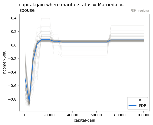
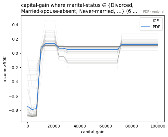
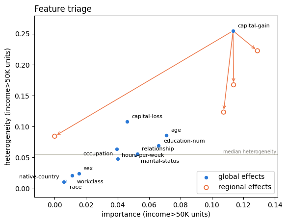
Look at the headline split: capital-gain
The global capital-gain curve has the dataset's famous cliff: predicted
probability jumps sharply once reported capital gains pass a few thousand
dollars (almost nobody with meaningful capital gains earned under $50K in
the 1994 census). The split shows the cliff is conditional — its height
depends on who is standing at it.
parts = pdp.find_regions("capital-gain", finder="best")
parts.show()
Feature 8 - Full partition tree:
🌳 Full Tree Structure:
───────────────────────
capital-gain 🔹 [id: 0 | heter: 0.25 | inst: 5000 | w: 1.00]
    marital-status = Married-civ-spouse 🔹 [id: 1 | heter: 0.23 | inst: 2319 | w: 0.46]
        education-num = 13.00 🔹 [id: 2 | heter: 0.17 | inst: 436 | w: 0.09]
        education-num ∈ {1.00, 2.00, 3.00, …} (15 levels) 🔹 [id: 3 | heter: 0.22 | inst: 1883 | w: 0.38]
    marital-status ∈ {Divorced, Married-spouse-absent, Never-married, …} (6 levels) 🔹 [id: 4 | heter: 0.21 | inst: 2681 | w: 0.54]
        age < 20.65 🔹 [id: 5 | heter: 0.08 | inst: 304 | w: 0.06]
        age ≥ 20.65 🔹 [id: 6 | heter: 0.12 | inst: 2377 | w: 0.48]
--------------------------------------------------
Feature 8 - Statistics per tree level:
🌳 Tree Summary:
─────────────────
Level 0🔹heter: 0.25
    Level 1🔹heter: 0.22 | 🔻0.04 (14.10%)
        Level 2🔹heter: 0.16 | 🔻0.06 (25.85%)
for r in parts:
    if r.level == 1:
        parts.plot(r.idx, centering=True)
effector.plot_triage(pdp, partitions={"capital-gain": parts})
Conclusion
- Classification needs no special machinery: wrap
predict_probawithadapters.classifier_probaand every verb — curves, regions, the ledger — works in probability units. - The ledger read is qualitatively different from the single-interaction
datasets: 72% → 86% takes four stacked splits, because the model's
probability surface interacts along several axes at once
(
education-num,capital-gain,capital-loss,hours-per-week— all conditioned onage/marital-status/capital-gain). - For a model like this, the final CALM — a small collection of region-conditional curves — is a far more faithful mental model than any single set of global curves.
Cross-method sanity check
The one-liner effector.explain with every engine this notebook's model
supports. A gradient-boosted tree is piecewise-constant, so derivative-scale
methods (RHALE, DerPDP) have no meaningful gradients to work with and are out
of scope here; PDP, ALE and SHAP-DP cover the output-scale reads. Where
methods disagree — ranking, accepted splits, R² — that is a property of the
data/model worth a closer look, not an error.
from pathlib import Path
_out = Path("reports") / "07_adult_income"
_out.mkdir(parents=True, exist_ok=True)

# === cross-method sweep: effector.explain on every applicable engine ======
sweep_reports = {}
for _m in ["pdp", "ale", "shapdp"]:
    _kw = {"nof_instances": 300} if _m == "shapdp" else {"nof_instances": 5000}
    print(f"--- {_m} " + "-" * 50)
    sweep_reports[_m] = effector.explain(
        data.x_train, model_forward, y=data.y_train, method=_m, schema=schema, **_kw
    )
    if _m != "pdp":  # the published report is the narrated one above
        sweep_reports[_m].to_html(_out / f"report_{_m}.html")

print()
print(f"{'method':<8} {'ranking (plotted)':<52} {'GAM R2':>8} {'final R2':>9}  splits")
for _m, _r in sweep_reports.items():
    _rank = " > ".join(fr.name for fr in _r.features)
    _ev = _r.explained_variance
    _sp = "; ".join(f"{s['name']} on {s['on']}" for s in _ev["stages"]) or "none"
    print(f"{_m:<8} {_rank:<52} {_ev['gam_r2']:>7.1%} {_ev['regional_r2']:>8.1%}  {_sp}")

print(f"\nreports stored in {_out}/")
--- pdp --------------------------------------------------


[effector] global effects   (GAM)  -> 72.5% of the model's variance
           regional effects (CALM) -> 86.0%
--- ale --------------------------------------------------


[effector] global effects   (GAM)  -> 75.3% of the model's variance
           regional effects (CALM) -> 82.9%


/home/givasile/github/packages/effector/effector/report.py:606: UserWarning: This figure includes Axes that are not compatible with tight_layout, so results might be incorrect.
  fig.tight_layout()


--- shapdp --------------------------------------------------


[effector] global effects   (GAM)  -> 64.2% of the model's variance
           regional effects (CALM) -> 73.5%


/home/givasile/github/packages/effector/effector/report.py:606: UserWarning: This figure includes Axes that are not compatible with tight_layout, so results might be incorrect.
  fig.tight_layout()


method   ranking (plotted)                                      GAM R2  final R2  splits
pdp      capital-gain > age > education-num > capital-loss > relationship > hours-per-week   72.5%    86.0%  education-num on age, capital-gain, marital-status; capital-gain on age, education-num, marital-status; capital-loss on age, capital-gain, marital-status; hours-per-week on age, capital-gain, marital-status
ale      capital-gain > education-num > capital-loss > relationship > marital-status > hours-per-week   75.3%    82.9%  education-num on age, capital-gain, marital-status; hours-per-week on age, capital-gain, relationship
shapdp   capital-gain > education-num > relationship > marital-status > age > capital-loss   64.2%    73.5%  capital-gain on marital-status, workclass; education-num on marital-status; capital-loss on education-num, relationship

reports stored in reports/07_adult_income/