Regional Effects (known black-box function)

• Author: givasile
• Runtime: ~20 s
• Description: A gentle introduction to regional effects: PDP, RHALE and SHAP-DP and their regional counterparts applied to a known black-box function with an interaction term, under uncorrelated and correlated features.
• 📄 The whole notebook in one page: PDP report

This tutorial provides a gentle overview of Regional Effect methods and introduces the Effector package. Regional Effects serve as a bridge between local and global feature effects. Αs shown in REPID, regional effect methods split the feature space in subregions where the feature interactions are minimized.

In this tutorial, we show how to use Effector to explain a black box function using regional effect plots. The tutorial is organized as follows:

• Introduction of the simulation example, using two datasets, one with uncorrelated and the other with correlated features.
• Examine how PDP/RHALE/SHAP plots model the feature effect and how their regional counterpart can minimize feature interactions, providing better explanations.
• Show how each of these methods behaves under correlated and uncorrelated features.

import numpy as np
import effector

Simulation example

Data Generating Distribution

We will generate \(N=1000\) examples with \(D=3\) features, which are uniformly distributed as follows:

Feature	Description	Distribution
\(x_1\)	Uniformly distributed between \(-1\) and \(1\)	\(x_1 \sim \mathcal{U}(-1,1)\)
\(x_2\)	Uniformly distributed between \(-1\) and \(1\)	\(x_2 \sim \mathcal{U}(-1,1)\)
\(x_3\)	Uniformly distributed between \(-1\) and \(1\)	\(x_3 \sim \mathcal{U}(-1,1)\)

For the correlated setting we keep the distributional assumptions for \(x_2\) and \(x_3\) but define \(x_1\) such that it is identical to \(x_3\) by: \(x_1 = x_3\).

def generate_dataset_uncorrelated(N):
    x1 = np.random.uniform(-1, 1, size=N)
    x2 = np.random.uniform(-1, 1, size=N)
    x3 = np.random.uniform(-1, 1, size=N)
    return np.stack((x1, x2, x3), axis=-1)

def generate_dataset_correlated(N):
    x3 = np.random.uniform(-1, 1, size=N)
    x2 = np.random.uniform(-1, 1, size=N)
    x1 = x3
    return np.stack((x1, x2, x3), axis=-1)

# generate the dataset for the uncorrelated and correlated setting
N = 1000
X_uncor_train = generate_dataset_uncorrelated(N)
X_uncor_test = generate_dataset_uncorrelated(10000)
X_cor_train = generate_dataset_correlated(N)
X_cor_test = generate_dataset_correlated(10000)

Black-box function

We will use the following linear model with a subgroup-specific interaction term: $$ y = 3x_1I_{x_3>0} - 3x_1I_{x_3\leq0} + x_3$$

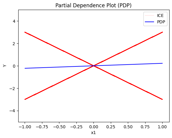
On a global level, there is a high heterogeneity for the features \(x_1\) and \(x_3\) due to their interaction with each other. However, this heterogeneity vanishes to 0 if the feature space is separated into subregions:

| Feature | Region | Average Effect | Heterogeneity | |---------|-------------|----------------|---------------| | $x_1$ | $x_3>0$ | $3x_1$ | 0 | | $x_1$ | $x_3\leq 0$ | $-3x_1$ | 0 | | $x_2$ | all | 0 | 0 | | $x_3$ | $x_3>0$ | $x_3$ | 0 | | $x_3$ | $x_3\leq 0$ | $x_3$ | 0 |

def model(x):
    f = np.where(x[:,2] > 0, 3*x[:,0] + x[:,2], -3*x[:,0] + x[:,2])
    return f

def model_jac(x):
    dy_dx = np.zeros_like(x)

    ind1 = x[:, 2] > 0
    ind2 = x[:, 2] <= 0

    dy_dx[ind1, 0] = 3
    dy_dx[ind2, 0] = -3
    dy_dx[:, 2] = 1
    return dy_dx

Y_uncor_train = model(X_uncor_train)
Y_uncor_test = model(X_uncor_test)
Y_cor_train = model(X_cor_train)
Y_cor_test = model(X_cor_test)      

---

PDP

The PDP is defined as the average of the model's output over the entire dataset, while varying the feature of interest.:

\[ \text{PDP}(x_s) = \mathbb{E}_{x_c}[f(x_s, x_c)] \]

and is approximated using the training data:

\[ \hat{\text{PDP}}(x_s) = \frac{1}{N} \sum_{j=1}^N f(x_s, x^{(i)}_c) = \frac{1}{N} \sum_{j=1}^N ICE^i(x_s)\]

The PDP is simply the average over the underlying ICE curves (local effects). The ICE curves show how the feature of interest influences the prediction of the ML model for each single instance. The ICE curves show the heterogeneity of the local effects.

Uncorrelated setting

Global PDP

pdp = effector.PDP(data=X_uncor_train, model=model, schema={"feature_names": ['x1','x2','x3'], "target_name": "Y"})
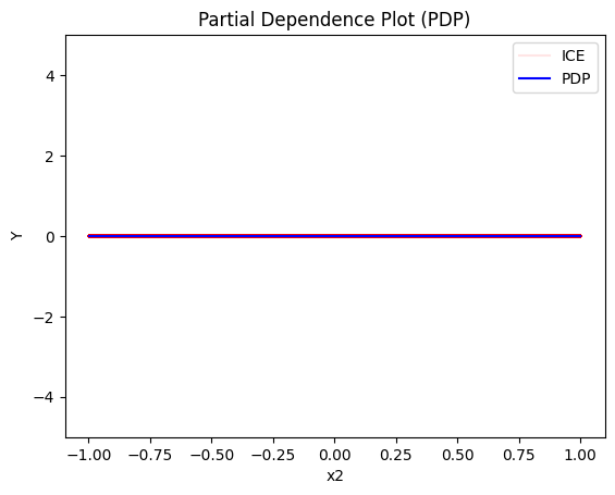
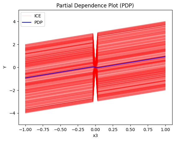
[pdp.plot(feature=i, centering=True, show_avg_output=False, heterogeneity="ice", y_limits=[-5, 5]) for i in range(3)]

[None, None, None]

Feature importance and the one-click report

Before drilling into regional effects manually, we can let effector rank the features for us. importances() returns, per feature, the dispersion of the mean effect — the \(\mu\)-twin of heterogeneity. effector.explain(...) runs the whole pipeline in one call: rank features by importance, plot the top ones, and automatically find_regions on the heterogeneous ones, returning a serializable Report.

# per-feature importance (mean-effect dispersion); x1 and x3 carry the interaction
print("PDP importances [x1, x2, x3]:", np.round(pdp.importances(), 3))

# one-click auto-explanation -> Report (values, serializable, self-contained HTML)
report = effector.explain(
    X_uncor_train, model, method="pdp",
    schema={"feature_names": ['x1', 'x2', 'x3'], "target_name": "Y"},
    nof_instances="all",
)
report.show()

# the whole notebook, in one page: the report published with this example
from pathlib import Path
_out = Path("reports") / "03_regional_effects_synthetic_f"
_out.mkdir(parents=True, exist_ok=True)
report.to_html(_out / "report_pdp.html")

PDP importances [x1, x2, x3]: [0.045 0.    0.573]
[effector] global effects   (GAM)  -> 10.4% of the model's variance
           regional effects (CALM) -> 100.0%

  ════════════════════════════════════════════════════════════════════════
  PDP report  ·  target: Y
  ════════════════════════════════════════════════════════════════════════

  DATA & MODEL
  ────────────────────────────────────────────────────────────────────────
    instances     1,000
    features      3  ·  3 continuous
    model output  mean -0.048 · std 1.84 · range [-3.93, 3.82]

  EXPLAINED VARIANCE
  ────────────────────────────────────────────────────────────────────────
    step         split on                 solo     ΔR²      R²       heter
    ──────────────────────────────────────────────────────────────────────
    GAM          (all features global)       —       —   10.4%           —
  + x1           x3                     +89.6%  +89.6%  100.0% 1.74 → 0.00
    ──────────────────────────────────────────────────────────────────────
    FINAL                                               100.0%

  REJECTED SPLITS                                            min gain 1.0%
  ────────────────────────────────────────────────────────────────────────
    feature      split on                 solo     ΔR²    reason
    ──────────────────────────────────────────────────────────────────────
  ✗ x3           x1                     +83.6%  -82.4%    redundant

    ✗ redundant: it would explain variance on its own (see solo),
      but the accepted splits already account for it.

  FEATURES                                ranked, in the selected snapshot
  ────────────────────────────────────────────────────────────────────────
    feature        importance                          heter      #regions
    ──────────────────────────────────────────────────────────────────────
    x1                 1.7402  ██████████████████     0.0000             2
    x3                 0.5731  ██████                 1.7403             1
    ──────────────────────────────────────────────────────────────────────
    the features above carry 100% of the total importance mass



Feature 0 - Full partition tree:
🌳 Full Tree Structure:
───────────────────────
x1 🔹 [id: 0 | heter: 1.74 | inst: 1000 | w: 1.00]
    x3 < -0.00 🔹 [id: 1 | heter: 0.00 | inst: 513 | w: 0.51]
    x3 ≥ -0.00 🔹 [id: 2 | heter: 0.00 | inst: 487 | w: 0.49]
--------------------------------------------------
Feature 0 - Statistics per tree level:
🌳 Tree Summary:
─────────────────
Level 0🔹heter: 1.74
    Level 1🔹heter: 0.00 | 🔻1.74 (100.00%)




/home/givasile/github/packages/effector/effector/report.py:606: UserWarning: This figure includes Axes that are not compatible with tight_layout, so results might be incorrect.
  fig.tight_layout()

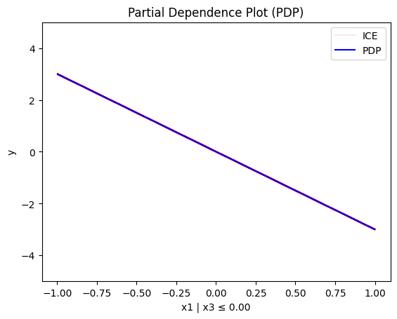
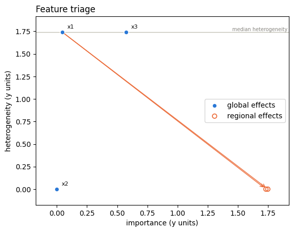
The same survey as one picture: effector.plot_triage puts importance on the x-axis and heterogeneity on the y-axis. Here x1 lands top-left — its global mean effect is flat (near-zero importance) yet its heterogeneity is the highest of all features: the +3/-3 slopes cancel in the average. That corner is exactly where find_regions pays off — the effect is hiding, not absent.

effector.plot_triage(pdp)

Regional PDP

Regional PDP will search for explanations that minimize the interaction-related heterogeneity.

# Regional effects are queried from the *global* effect via `find_regions`,
# which returns `Partition` value objects (nothing is stored on the effect).
# Here we use the *plural* form, `find_regions(features=...)`: one call that
# runs the search per feature and returns a `{feature_name: Partition}` dict
# (`features` also accepts "heterogeneous" to target only the features whose
# heter_score is at or above the median).
pdp = effector.PDP(
    data=X_uncor_train, model=model,
    schema={"feature_names": ['x1', 'x2', 'x3']},
    axis_limits=np.array([[-1, 1], [-1, 1], [-1, 1]]).T,
    nof_instances="all",
)
pdp.fit("all", centering=True)

finder = effector.space_partitioning.Best(min_heterogeneity_decrease_pcg=0.3, numerical_features_grid_size=10)
parts = pdp.find_regions(features="all", finder=finder)  # {name: Partition} — the plural form
partitions = [parts[name] for name in ["x1", "x2", "x3"]]

partitions[0].show()

Feature 0 - Full partition tree:
🌳 Full Tree Structure:
───────────────────────
x1 🔹 [id: 0 | heter: 1.74 | inst: 1000 | w: 1.00]
    x3 < 0.00 🔹 [id: 1 | heter: 0.00 | inst: 513 | w: 0.51]
    x3 ≥ 0.00 🔹 [id: 2 | heter: 0.00 | inst: 487 | w: 0.49]
--------------------------------------------------
Feature 0 - Statistics per tree level:
🌳 Tree Summary:
─────────────────
Level 0🔹heter: 1.74
    Level 1🔹heter: 0.00 | 🔻1.74 (100.00%)

[partitions[0].plot(idx, heterogeneity="ice", centering=True, y_limits=[-5, 5]) for idx in [1, 2]]

[None, None]

partitions[1].show()

Feature 1 - Full partition tree:
No splits found for feature 1
--------------------------------------------------
Feature 1 - Statistics per tree level:
No splits found for feature 1

partitions[2].show()

Feature 2 - Full partition tree:
🌳 Full Tree Structure:
───────────────────────
x3 🔹 [id: 0 | heter: 1.74 | inst: 1000 | w: 1.00]
    x1 < 0.00 🔹 [id: 1 | heter: 0.85 | inst: 502 | w: 0.50]
        x1 < -0.60 🔹 [id: 2 | heter: 0.34 | inst: 202 | w: 0.20]
        -0.60 ≤ x1 < 0.00 🔹 [id: 3 | heter: 0.51 | inst: 300 | w: 0.30]
    x1 ≥ 0.00 🔹 [id: 4 | heter: 0.86 | inst: 498 | w: 0.50]
        0.00 ≤ x1 < 0.60 🔹 [id: 5 | heter: 0.51 | inst: 288 | w: 0.29]
        x1 ≥ 0.60 🔹 [id: 6 | heter: 0.37 | inst: 210 | w: 0.21]
--------------------------------------------------
Feature 2 - Statistics per tree level:
🌳 Tree Summary:
─────────────────
Level 0🔹heter: 1.74
    Level 1🔹heter: 0.86 | 🔻0.88 (50.63%)
        Level 2🔹heter: 0.44 | 🔻0.41 (48.25%)

partitions[2].plot(1, heterogeneity="ice", centering=True, y_limits=[-5, 5])
partitions[2].plot(2, heterogeneity="ice", centering=True, y_limits=[-5, 5])

Triage, after: with partitions= the same plane shows the before→after story — arrows run from x1's global point to its leaves. Both leaves jump right (within each subregion the effect is strongly decisive, |slope| = 3) and down (the heterogeneity is explained). A hidden effect became two visible ones.

effector.plot_triage(pdp, partitions={"x1": partitions[0]})

Conclusion

For the Global PDP:

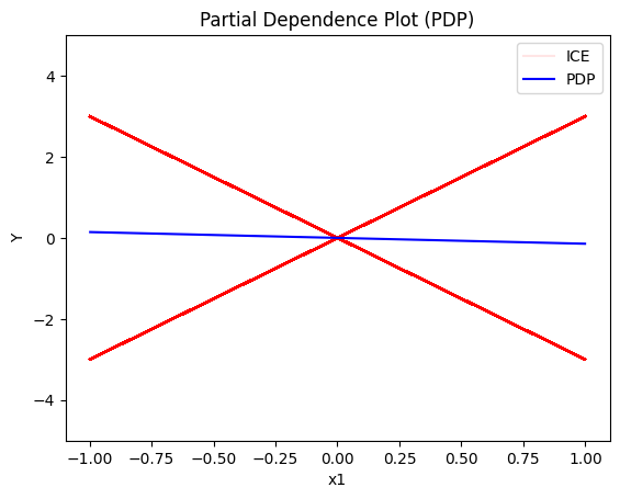
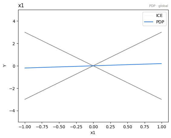
• the average effect of \(x_1\) is \(0\) with some heterogeneity implied by the interaction with \(x_1\). The heterogeneity is expressed with two opposite lines; \(-3x_1\) when \(x_1 \leq 0\) and \(3x_1\) when \(x_1 >0\)
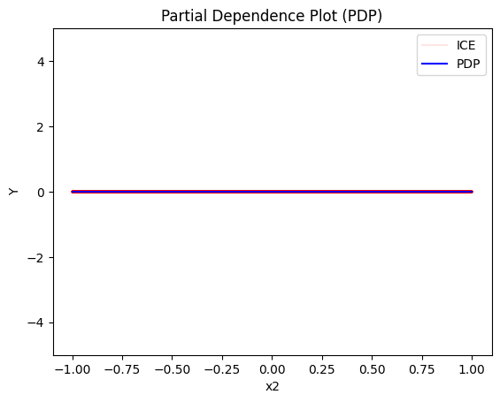
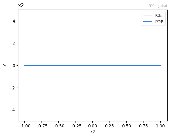
• the average effect of \(x_2\) to be \(0\) without heterogeneity
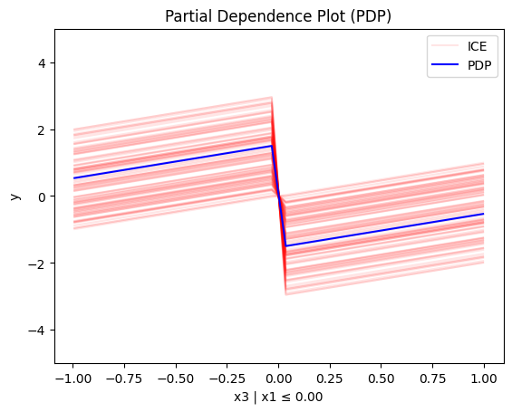
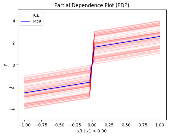
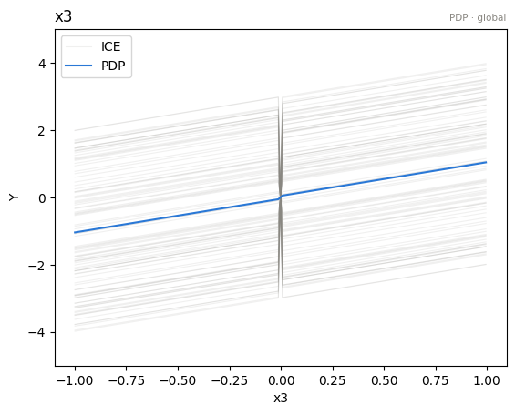
• the average effect of \(x_3\) to be \(x_3\) with some heterogeneity due to the interaction with \(x_1\). The heterogeneity is expressed with a discontinuity around \(x_3=0\), with either a positive or a negative offset depending on the value of \(x_1^i\)

---

For the Regional PDP:

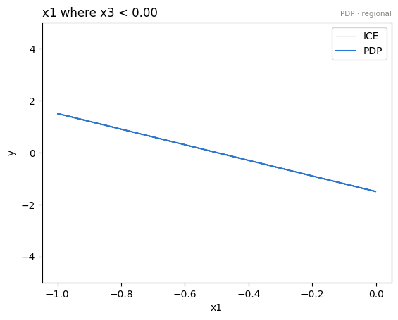
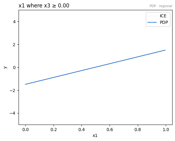
• For \(x_1\), the algorithm finds two regions, one for \(x_3 \leq 0\) and one for \(x_3 > 0\)
• when \(x_3>0\) the effect is \(3x_1\)
• when \(x_3 \leq 0\), the effect is \(-3x_1\)
• For \(x_2\) the algorithm does not find any subregion
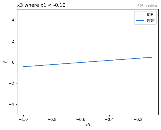
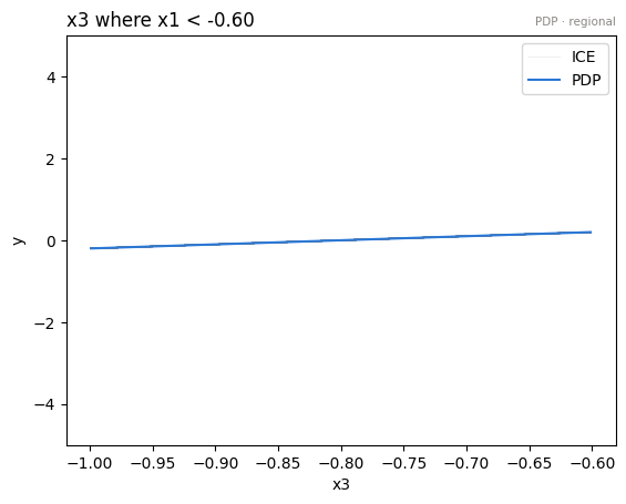
• For \(x_3\), there is a change in the offset:
• when \(x_1>0\) the line is \(x_3 - 3x_1^i\) in the first half and \(x_3 + 3x_1^i\) later
• when \(x_1<0\) the line is \(x_3 + 3x_1^i\) in the first half and \(x_3 - 3x_1^i\) later

Correlated setting

PDP assumes feature independence, therefore, it is not a good explanation method for the correlated case. Due to this face, we expect the explanations to be identical with the uncorrelated case, which is not correct as we will see later in (RH)ALE plots.

Global PDP

pdp = effector.PDP(data=X_cor_train, model=model, schema={"feature_names": ['x1','x2','x3'], "target_name": "Y"})
[pdp.plot(feature=i, centering=True, show_avg_output=False, heterogeneity="ice", y_limits=[-5, 5]) for i in range(3)]

[None, None, None]

Regional-PDP

pdp = effector.PDP(
    data=X_cor_train, model=model,
    schema={"feature_names": ['x1', 'x2', 'x3']},
    axis_limits=np.array([[-1, 1], [-1, 1], [-1, 1]]).T,
    nof_instances="all",
)
pdp.fit("all", centering=True)

# finder="best" is the default Best() partitioner
partitions = {feat: pdp.find_regions(feat, finder="best") for feat in range(3)}

partitions[0].show()

Feature 0 - Full partition tree:
🌳 Full Tree Structure:
───────────────────────
x1 🔹 [id: 0 | heter: 1.75 | inst: 1000 | w: 1.00]
    x3 < 0.00 🔹 [id: 1 | heter: 0.00 | inst: 467 | w: 0.47]
    x3 ≥ 0.00 🔹 [id: 2 | heter: 0.00 | inst: 533 | w: 0.53]
--------------------------------------------------
Feature 0 - Statistics per tree level:
🌳 Tree Summary:
─────────────────
Level 0🔹heter: 1.75
    Level 1🔹heter: 0.00 | 🔻1.75 (100.00%)

partitions[0].plot(1, heterogeneity="ice", centering=True, y_limits=[-5, 5])
partitions[0].plot(2, heterogeneity="ice", centering=True, y_limits=[-5, 5])

partitions[1].show()

Feature 1 - Full partition tree:
No splits found for feature 1
--------------------------------------------------
Feature 1 - Statistics per tree level:
No splits found for feature 1

partitions[2].show()

Feature 2 - Full partition tree:
🌳 Full Tree Structure:
───────────────────────
x3 🔹 [id: 0 | heter: 1.75 | inst: 1000 | w: 1.00]
    x1 < -0.10 🔹 [id: 1 | heter: 0.81 | inst: 415 | w: 0.41]
        x1 < -0.60 🔹 [id: 2 | heter: 0.34 | inst: 215 | w: 0.21]
        -0.60 ≤ x1 < -0.10 🔹 [id: 3 | heter: 0.42 | inst: 200 | w: 0.20]
    x1 ≥ -0.10 🔹 [id: 4 | heter: 0.93 | inst: 585 | w: 0.58]
        -0.10 ≤ x1 < 0.40 🔹 [id: 5 | heter: 0.42 | inst: 274 | w: 0.27]
        x1 ≥ 0.40 🔹 [id: 6 | heter: 0.51 | inst: 311 | w: 0.31]
--------------------------------------------------
Feature 2 - Statistics per tree level:
🌳 Tree Summary:
─────────────────
Level 0🔹heter: 1.75
    Level 1🔹heter: 0.88 | 🔻0.87 (49.86%)
        Level 2🔹heter: 0.43 | 🔻0.44 (50.69%)

partitions[2].plot(1, heterogeneity="ice", centering=True, y_limits=[-5, 5])
partitions[2].plot(2, heterogeneity="ice", centering=True, y_limits=[-5, 5])

Conclusion

As expected, the global and the regional PDP explanations are identical with the uncorrelated case.

(RH)ALE

(RH)ALE defines the feature effect as the integral of the partial derivative of the model's output with respect to the feature of interest:

\[\text{ALE}(x_s) = \int_{z=0}^{x_s} \mathbb{E}_{x_c|x_s=z}\left [ \frac{\partial f}{\partial x_s} (z, x_c) \right ] \partial z\]

The approximation is defined as:

\[\hat{\text{ALE}}(x_s) = \sum_{k=1}^{k_{x_s}} \frac{1}{| \mathcal{S}_k |} \sum_{i: x^{(i)} \in \mathcal{S}_k} \left [ f(z_k, x_c) - f(z_{k-1}, x_c) \right ]\]

\(\hat{\text{ALE}}(x_s)\) uses a Riemannian sum to approximate the integral of \(\text{ALE}(x_s)\). The axis of the \(s\)-th feature is split in \(K\) bins (intervals) of equal size. In each bin, the average effect of the feature of interest is estimated using the instances that fall in the bin. The average effect in each bin is called bin-effect.

Robust and Heterogeneity-aware ALE (RHALE) is a variant of ALE, proposed by Gkolemis et. al, where the local effects are computed using automatic differentiation:

\[\hat{\text{RHALE}}(x_s) = \sum_{k=1}^{k_{x_s}} \frac{1}{ \left | \mathcal{S}_k \right |} \sum_{i: x^{(i)} \in \mathcal{S}_k} \frac{\partial f}{\partial x_s} (x_s^{(i)}, x_c^{(i)})\]

In their paper, Gkolemis et. al showed that RHALE has specific advantages over ALE: (a) it ensures on-distribution sampling (b) an unbiased estimation of the heterogeneity and (c) an optimal trade-off between bias and variance. In our example, we will use the RHALE approximation.

Uncorrelated setting

Global RHALE

rhale = effector.RHALE(data=X_uncor_train, model=model, model_jac=model_jac, schema={"feature_names": ['x1','x2','x3'], "target_name": "Y"})

binning_method = effector.axis_partitioning.Fixed(10, min_points_per_bin=0)
rhale.fit(features="all", binning_method=binning_method, centering=True)

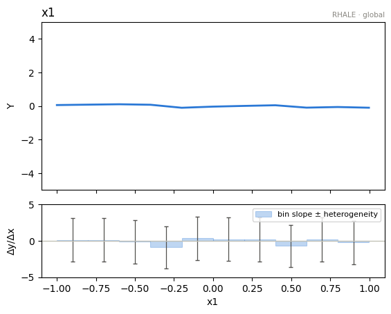
rhale.plot(feature=0, centering=True, heterogeneity="std", show_avg_output=False, y_limits=[-5, 5], dy_limits=[-5, 5])
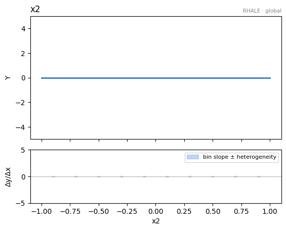
rhale.plot(feature=1, centering=True, heterogeneity="std", show_avg_output=False, y_limits=[-5, 5], dy_limits=[-5, 5])
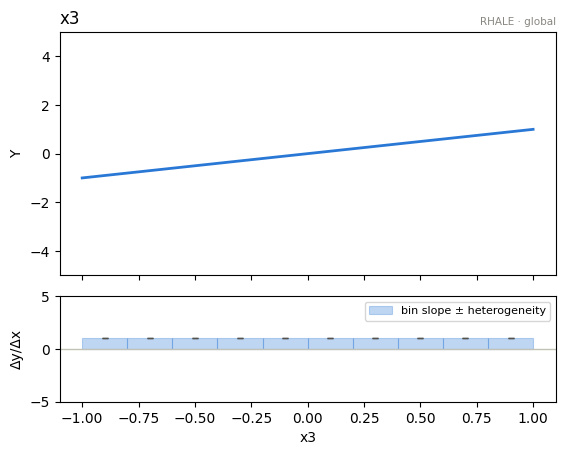
rhale.plot(feature=2, centering=True, heterogeneity="std", show_avg_output=False, y_limits=[-5, 5], dy_limits=[-5, 5])

Regional RHALE

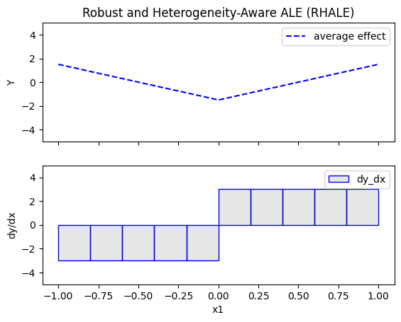
The disadvantage of RHALE plot is that it does not reveal the type of heterogeneity. Therefore, Regional (RH)ALE plots are very helpful to identify the type of heterogeneity. Let's see that in practice:

rhale = effector.RHALE(
    data=X_uncor_train, model=model, model_jac=model_jac,
    schema={"feature_names": ['x1', 'x2', 'x3']},
    axis_limits=np.array([[-1, 1], [-1, 1], [-1, 1]]).T,
    nof_instances="all",
)
binning_method = effector.axis_partitioning.Fixed(11, min_points_per_bin=0)
rhale.fit("all", binning_method=binning_method, centering=True)

finder = effector.space_partitioning.Best(min_heterogeneity_decrease_pcg=0.3, numerical_features_grid_size=10)
partitions = {feat: rhale.find_regions(feat, finder=finder) for feat in range(3)}

partitions[0].show()

Feature 0 - Full partition tree:
🌳 Full Tree Structure:
───────────────────────
x1 🔹 [id: 0 | heter: 1.73 | inst: 1000 | w: 1.00]
    x3 < 0.00 🔹 [id: 1 | heter: 0.00 | inst: 513 | w: 0.51]
    x3 ≥ 0.00 🔹 [id: 2 | heter: 0.00 | inst: 487 | w: 0.49]
--------------------------------------------------
Feature 0 - Statistics per tree level:
🌳 Tree Summary:
─────────────────
Level 0🔹heter: 1.73
    Level 1🔹heter: 0.00 | 🔻1.73 (100.00%)

partitions[0].plot(1, heterogeneity="std", centering=True, y_limits=[-5, 5])
partitions[0].plot(2, heterogeneity="std", centering=True, y_limits=[-5, 5])

partitions[1].show()

Feature 1 - Full partition tree:
No splits found for feature 1
--------------------------------------------------
Feature 1 - Statistics per tree level:
No splits found for feature 1

partitions[2].show()

Feature 2 - Full partition tree:
No splits found for feature 2
--------------------------------------------------
Feature 2 - Statistics per tree level:
No splits found for feature 2

Conclusion

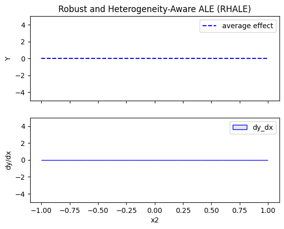
The explanations are similar to the ones obtained with the PDP plots. The average effect of \(x_1\) is \(0\) with some heterogeneity due to the interaction with \(x_1\). The heterogeneity is shown with the red vertical bars. The average effect of \(x_2\) is \(0\) without heterogeneity. The average effect of \(x_3\) is \(x_3\), but in contrast with the PDP plots, there is no heterogeneity. The regional RHALE plots explain the type of the heterogeneity for \(x_1\).

Correlated setting

In the correlated setting \(x_3=x_1\), therefore the model's formula becomes:

$$ y = 3x_1I_{x_1>0} - 3x_1I_{x_1\leq0} + x_3$$

Global RHALE

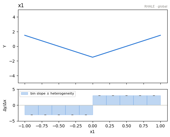
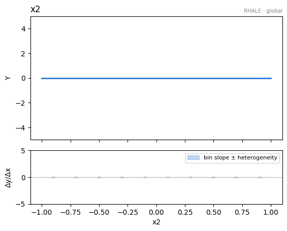
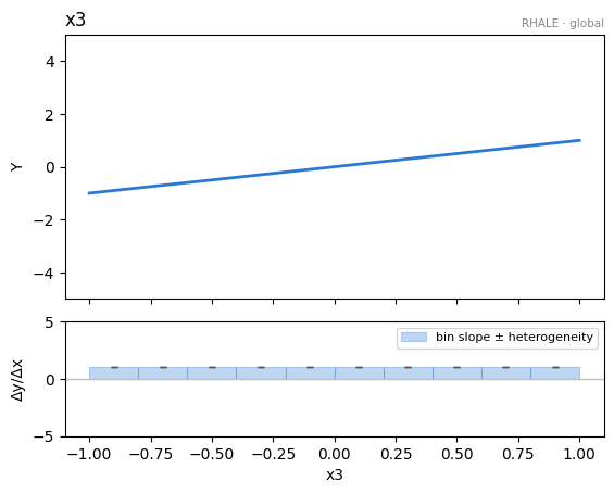
RHALE plots respect feature correlations, therefore we expect the explanations to follow the formula above.

rhale = effector.RHALE(data=X_cor_train, model=model, model_jac=model_jac, 
                       schema={"feature_names": ['x1','x2','x3'], "target_name": "Y"}, 
                       axis_limits=np.array([[-1, 1], [-1, 1], [-1, 1]]).T)
binning_method = effector.axis_partitioning.Fixed(10, min_points_per_bin=0)
rhale.fit(features="all", binning_method=binning_method, centering=True)

[rhale.plot(feature=i, show_avg_output=False, y_limits=[-5, 5], dy_limits=[-5, 5]) for i in range(3)]

[None, None, None]

Regional RHALE

rhale = effector.RHALE(
    data=X_cor_train, model=model, model_jac=model_jac,
    schema={"feature_names": ['x1', 'x2', 'x3']},
    axis_limits=np.array([[-1, 1], [-1, 1], [-1, 1]]).T,
    nof_instances="all",
)
binning_method = effector.axis_partitioning.Fixed(10, min_points_per_bin=0)
rhale.fit("all", binning_method=binning_method, centering=True)

finder = effector.space_partitioning.Best(min_heterogeneity_decrease_pcg=0.3, numerical_features_grid_size=10)
partitions = {feat: rhale.find_regions(feat, finder=finder) for feat in range(3)}

partitions[0].show()

Feature 0 - Full partition tree:
No splits found for feature 0
--------------------------------------------------
Feature 0 - Statistics per tree level:
No splits found for feature 0

partitions[1].show()

Feature 1 - Full partition tree:
No splits found for feature 1
--------------------------------------------------
Feature 1 - Statistics per tree level:
No splits found for feature 1

partitions[2].show()

Feature 2 - Full partition tree:
No splits found for feature 2
--------------------------------------------------
Feature 2 - Statistics per tree level:
No splits found for feature 2

Conclusion

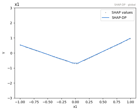
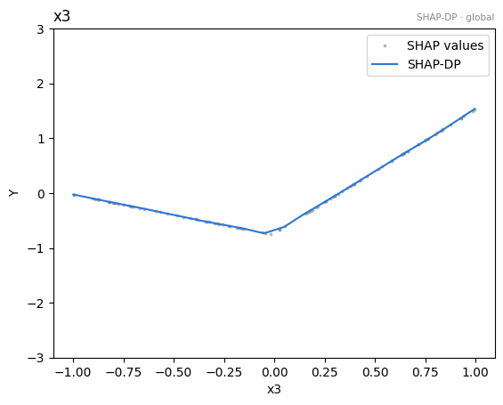
The global RHALE plots follow the formula obtained after setting \(x_1=x_3\) while the Regional (RH)ALE plot do not find any subregions in the correlated case.

SHAP DP

Uncorrelated setting

Global SHAP DP

shap = effector.ShapDP(data=X_uncor_train, model=model, schema={"feature_names": ['x1','x2','x3'], "target_name": "Y"})
binning_method = effector.axis_partitioning.Fixed(nof_bins=5, min_points_per_bin=0)
shap.fit("all", binning_method=binning_method)
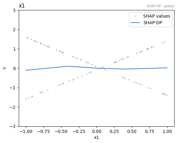
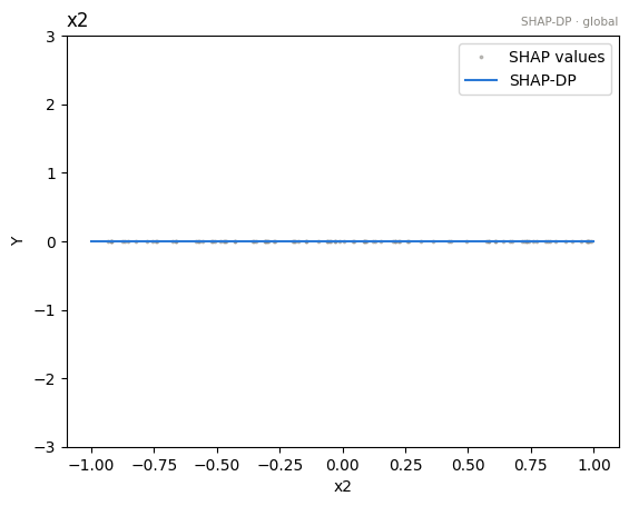
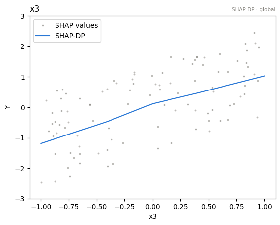
[shap.plot(feature=i, show_avg_output=False, y_limits=[-3, 3]) for i in range(3)]

[None, None, None]

Regional SHAP-DP

shap = effector.ShapDP(
    data=X_uncor_train, model=model,
    schema={"feature_names": ['x1', 'x2', 'x3']},
    axis_limits=np.array([[-1, 1], [-1, 1], [-1, 1]]).T,
    nof_instances="all",
)
shap.fit("all", binning_method=effector.axis_partitioning.Fixed(nof_bins=5, min_points_per_bin=0))

finder = effector.space_partitioning.Best(min_heterogeneity_decrease_pcg=0.6, numerical_features_grid_size=10)
partitions = {feat: shap.find_regions(feat, finder=finder) for feat in range(3)}

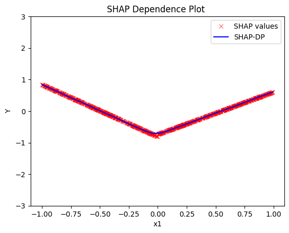
partitions[0].show()

Feature 0 - Full partition tree:
🌳 Full Tree Structure:
───────────────────────
x1 🔹 [id: 0 | heter: 0.90 | inst: 1000 | w: 1.00]
    x3 < 0.00 🔹 [id: 1 | heter: 0.17 | inst: 513 | w: 0.51]
    x3 ≥ 0.00 🔹 [id: 2 | heter: 0.17 | inst: 487 | w: 0.49]
--------------------------------------------------
Feature 0 - Statistics per tree level:
🌳 Tree Summary:
─────────────────
Level 0🔹heter: 0.90
    Level 1🔹heter: 0.17 | 🔻0.73 (80.85%)

partitions[0].plot(1, heterogeneity="std", centering=True, y_limits=[-5, 5])
partitions[0].plot(2, heterogeneity="std", centering=True, y_limits=[-5, 5])

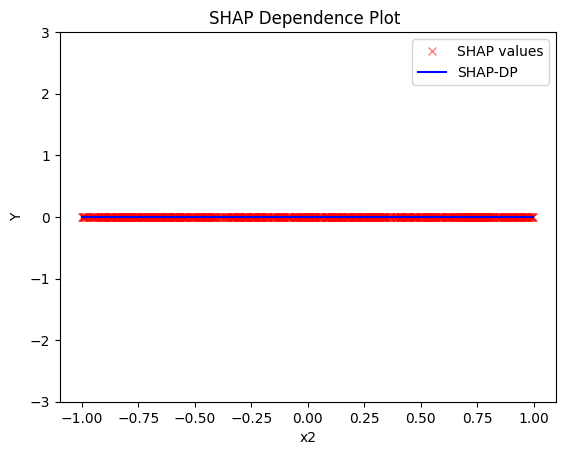
partitions[1].show()

Feature 1 - Full partition tree:
No splits found for feature 1
--------------------------------------------------
Feature 1 - Statistics per tree level:
No splits found for feature 1

partitions[2].show()

Feature 2 - Full partition tree:
No splits found for feature 2
--------------------------------------------------
Feature 2 - Statistics per tree level:
No splits found for feature 2

Conclusion

Global SHAP-DP:

• the average effect of \(x_1\) is \(0\) with some heterogeneity implied by the interaction with \(x_1\). The heterogeneity is expressed with two opposite lines; \(-3x_1\) when \(x_1 \leq 0\) and \(3x_1\) when \(x_1 >0\)
• the average effect of \(x_2\) to be \(0\) without heterogeneity
• the average effect of \(x_3\) to be \(x_3\) with some heterogeneity due to the interaction with \(x_1\). In contrast with other methods, SHAP spread the heterogeneity along the x-axis.

Regional SHAP-DP:

Correlated setting

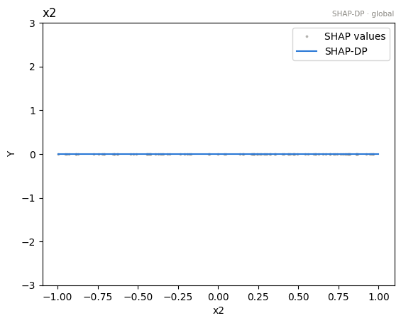
Global SHAP-DP

shap = effector.ShapDP(data=X_cor_train, model=model, schema={"feature_names": ['x1','x2','x3'], "target_name": "Y"})

[shap.plot(feature=i, y_limits=[-3, 3]) for i in range(3)]

[None, None, None]

Regional SHAP

shap = effector.ShapDP(
    data=X_cor_train, model=model,
    schema={"feature_names": ['x1', 'x2', 'x3']},
    axis_limits=np.array([[-1, 1], [-1, 1], [-1, 1]]).T,
    nof_instances="all",
)
shap.fit("all")

finder = effector.space_partitioning.Best(min_heterogeneity_decrease_pcg=0.6, numerical_features_grid_size=10)
partitions = {feat: shap.find_regions(feat, finder=finder) for feat in range(3)}

partitions[0].show()

Feature 0 - Full partition tree:
No splits found for feature 0
--------------------------------------------------
Feature 0 - Statistics per tree level:
No splits found for feature 0

partitions[1].show()

Feature 1 - Full partition tree:
No splits found for feature 1
--------------------------------------------------
Feature 1 - Statistics per tree level:
No splits found for feature 1

partitions[2].show()

Feature 2 - Full partition tree:
No splits found for feature 2
--------------------------------------------------
Feature 2 - Statistics per tree level:
No splits found for feature 2

Cross-method sanity check

The one-liner effector.explain with every engine this notebook's model supports. Everything must run end to end; the closing table puts the reads side by side. Where methods disagree — ranking, accepted splits, R² — that is a property of the data/model worth a closer look, not an error.

from pathlib import Path
_out = Path("reports") / "03_regional_effects_synthetic_f"
_out.mkdir(parents=True, exist_ok=True)

# === cross-method sweep: effector.explain on every applicable engine ======
sweep_reports = {}
for _m in ["pdp", "derpdp", "ale", "rhale", "shapdp"]:
    _kw = {"nof_instances": 300} if _m == "shapdp" else {}
    print(f"--- {_m} " + "-" * 50)
    sweep_reports[_m] = effector.explain(
        X_uncor_train, model, model_jac, method=_m, schema={"feature_names": ['x1','x2','x3'], "target_name": "Y"}, **_kw
    )
    if _m != "pdp":  # the published report is the narrated one above
        sweep_reports[_m].to_html(_out / f"report_{_m}.html")

print()
print(f"{'method':<8} {'ranking (plotted)':<44} {'GAM R2':>8} {'final R2':>9}  splits")
for _m, _r in sweep_reports.items():
    _rank = " > ".join(fr.name for fr in _r.features)
    _ev = _r.explained_variance
    if _ev:
        _sp = "; ".join(f"{s['name']} on {s['on']}" for s in _ev["stages"]) or "none"
        print(f"{_m:<8} {_rank:<44} {_ev['gam_r2']:>7.1%} {_ev['regional_r2']:>8.1%}  {_sp}")
    else:
        print(f"{_m:<8} {_rank:<44} {'-':>7} {'-':>8}  (derivative scale: no variance ledger)")

print(f"\nreports stored in {_out}/")

--- pdp --------------------------------------------------
[effector] global effects   (GAM)  -> 10.4% of the model's variance
           regional effects (CALM) -> 100.0%
--- derpdp --------------------------------------------------


/home/givasile/github/packages/effector/effector/report.py:606: UserWarning: This figure includes Axes that are not compatible with tight_layout, so results might be incorrect.
  fig.tight_layout()


--- ale --------------------------------------------------
[effector] global effects   (GAM)  -> 6.1% of the model's variance
           regional effects (CALM) -> 99.8%


/home/givasile/github/packages/effector/effector/report.py:606: UserWarning: This figure includes Axes that are not compatible with tight_layout, so results might be incorrect.
  fig.tight_layout()


--- rhale --------------------------------------------------
[effector] global effects   (GAM)  -> 10.4% of the model's variance
           regional effects (CALM) -> 100.0%


/home/givasile/github/packages/effector/effector/report.py:606: UserWarning: This figure includes Axes that are not compatible with tight_layout, so results might be incorrect.
  fig.tight_layout()


--- shapdp --------------------------------------------------


[effector] global effects   (GAM)  -> 20.6% of the model's variance
           regional effects (CALM) -> 98.4%


/home/givasile/github/packages/effector/effector/report.py:606: UserWarning: This figure includes Axes that are not compatible with tight_layout, so results might be incorrect.
  fig.tight_layout()



method   ranking (plotted)                              GAM R2  final R2  splits
pdp      x1 > x3                                        10.4%   100.0%  x1 on x3
derpdp   x3                                                 -        -  (derivative scale: no variance ledger)
ale      x1 > x3                                         6.1%    99.8%  x1 on x3
rhale    x1 > x3                                        10.4%   100.0%  x1 on x3
shapdp   x3 > x1                                        20.6%    98.4%  x1 on x2, x3; x3 on x1

reports stored in reports/03_regional_effects_synthetic_f/