Model with conditional interaction

• Author: givasile
• Runtime: ~25 s
• Description: How PDP, ALE and RHALE quantify the heterogeneity introduced by a conditional interaction; each heterogeneity estimate is derived analytically and tested against effector.benchmarks.
• 📄 The whole notebook in one page: PDP report

In this example, we show the heterogeneity of the global effects, using PDP, ALE, and RHALE, on a model with conditional interactions. We will use the following model:

\[ f(x_1, x_2, x_3) = -x_1^2 \mathbb{1}_{x_2 <0} + x_1^2 \mathbb{1}_{x_2 \geq 0} + e^{x_3} \]

where the features \(x_1, x_2, x_3\) are independent and uniformly distributed in the interval \([-1, 1]\). The model has an interaction between \(x_1\) and \(x_2\) caused by the terms: \(f_{1,2}(x_1, x_2) = -x_1^2 \mathbb{1}_{x_2 <0} + x_1^2 \mathbb{1}_{x_2 \geq 0}\). This means that the effect of \(x_1\) on the output \(y\) depends on the value of \(x_2\) and vice versa. Terms like this introduce heterogeneity. Each global effect method has a different formula for qunatifying such heterogeneity; below, we will see how PDP, ALE, and RHALE handles it.

In contrast, \(x_3\) does not interact with any other feature, so its global effect has zero heterogeneity.

import numpy as np
import matplotlib.pyplot as plt
import effector

np.random.seed(21)

bench = effector.benchmarks.ConditionalInteractionUniform()
model = bench.model
dataset = bench.dataset
x = bench.generate_data(10_000)

PDP

Effector

Let's see below the PDP heterogeneity for each feature, using effector.

pdp = effector.PDP(x, model.predict, axis_limits=dataset.axis_limits)
pdp.fit(features="all", centering=True)
for feature in [0, 1, 2]:
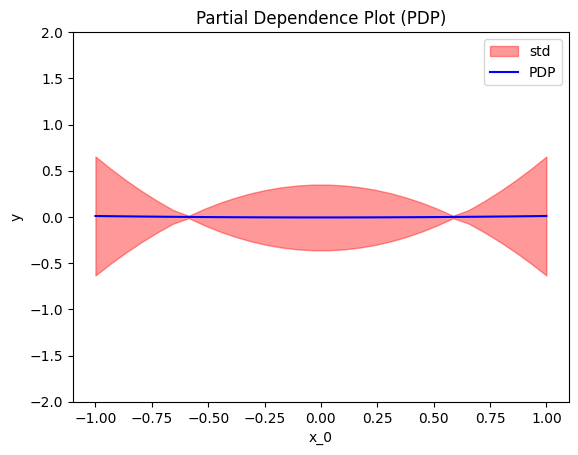
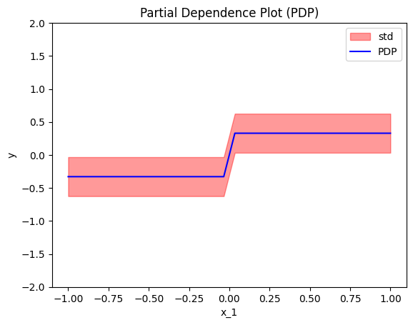
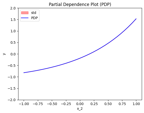
    pdp.plot(feature=feature, centering=True, heterogeneity=True, y_limits=[-2, 2])

for feature in [0, 1, 2]:
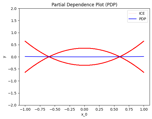
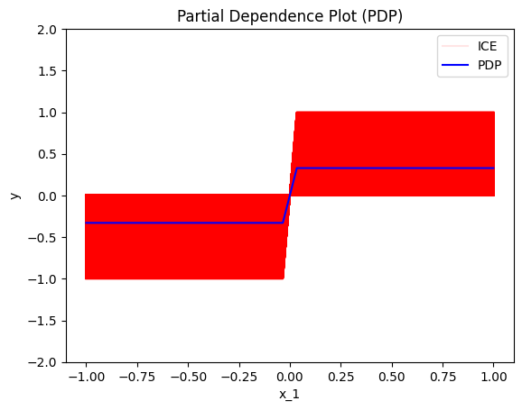
    pdp.plot(feature=feature, centering=True, heterogeneity="ice", y_limits=[-2, 2])

pdp = effector.PDP(x, model.predict, axis_limits=dataset.axis_limits, nof_instances="all")
pdp.fit(features="all", centering=True)
heter_per_feat = []
for feature in [0, 1, 2]:
    y_var = pdp.eval_heter(feature=feature, xs=np.linspace(-1, 1, 100))
    print(f"Heterogeneity of x_{feature}: {y_var.mean():.3f}")
    heter_per_feat.append(y_var.mean())

Heterogeneity of x_0: 0.094
Heterogeneity of x_1: 0.088
Heterogeneity of x_2: 0.000

Importance & one-click report (new API)

importances() is the \(\mu\)-twin of the heterogeneity above: instead of the dispersion of the local effects, it summarises the dispersion of the mean effect per feature (how much signal each feature carries). We also call effector.explain(...), which fits once, ranks features by importance, and returns a self-contained Report.

# per-feature importance = dispersion of the mean effect (the mu-twin of the
# heterogeneity we studied above); x_1 and x_2 should rank equally, x_3 near zero.
print("PDP importances:", np.round(pdp.importances(), 3))

# one-click auto-explanation -> Report (serializable; self-contained HTML)
report = effector.explain(
    x,
    model.predict,
    method="pdp",
    schema={"feature_names": ["x1", "x2", "x3"]},
    nof_instances="all",
)
report.show()

# the whole notebook, in one page: the report published with this example
from pathlib import Path
_out = Path("reports") / "05_conditional_interaction_independent_uniform_heter"
_out.mkdir(parents=True, exist_ok=True)
report.to_html(_out / "report_pdp.html")

PDP importances: [0.005 0.325 0.66 ]


[effector] global effects   (GAM)  -> 85.8% of the model's variance
           regional effects (CALM) -> 99.8%

  ════════════════════════════════════════════════════════════════════════
  PDP report  ·  target: y
  ════════════════════════════════════════════════════════════════════════

  DATA & MODEL
  ────────────────────────────────────────────────────────────────────────
    instances     10,000
    features      3  ·  3 continuous
    model output  mean 1.17 · std 0.79 · range [-0.601, 3.7]

  EXPLAINED VARIANCE
  ────────────────────────────────────────────────────────────────────────
    step         split on                 solo     ΔR²      R²       heter
    ──────────────────────────────────────────────────────────────────────
    GAM          (all features global)       —       —   85.8%           —
  + x1           x2                     +14.0%  +14.0%   99.8% 0.30 → 0.00
    ──────────────────────────────────────────────────────────────────────
    FINAL                                                99.8%

  REJECTED SPLITS                                            min gain 1.0%
  ────────────────────────────────────────────────────────────────────────
    feature      split on                 solo     ΔR²    reason
    ──────────────────────────────────────────────────────────────────────
  ✗ x2           x1                     +10.9%  -10.8%    redundant

    ✗ redundant: it would explain variance on its own (see solo),
      but the accepted splits already account for it.

  FEATURES                                ranked, in the selected snapshot
  ────────────────────────────────────────────────────────────────────────
    feature        importance                          heter      #regions
    ──────────────────────────────────────────────────────────────────────
    x3                 0.6603  ██████████████████     0.0000             1
    x2                 0.3253  █████████              0.2960             1
    x1                 0.2959  ████████               0.0000             2
    ──────────────────────────────────────────────────────────────────────
    the features above carry 100% of the total importance mass



Feature 0 - Full partition tree:
🌳 Full Tree Structure:
───────────────────────
x1 🔹 [id: 0 | heter: 0.30 | inst: 10000 | w: 1.00]
    x2 < -0.00 🔹 [id: 1 | heter: 0.00 | inst: 4922 | w: 0.49]
    x2 ≥ -0.00 🔹 [id: 2 | heter: 0.00 | inst: 5078 | w: 0.51]
--------------------------------------------------
Feature 0 - Statistics per tree level:
🌳 Tree Summary:
─────────────────
Level 0🔹heter: 0.30
    Level 1🔹heter: 0.00 | 🔻0.30 (100.00%)




/home/givasile/github/packages/effector/effector/report.py:606: UserWarning: This figure includes Axes that are not compatible with tight_layout, so results might be incorrect.
  fig.tight_layout()

Conclusions:

• The global effect of \(x_1\) arises from heterogenous local effects, as \(h(x_1) > 0\) for all \(x_1\). The std margins (red area of height \(\pm h(x_1)\) around the global effect) musleadingly suggest that the heterogeneity is minimized at \(x_1 = \pm \frac{2}{3}\). ICE provide a clearer picture; they reveal two groups of effects, \(-x_1^2 + c_1\) and \(x_1^2 + c_2\). The heterogeneity as a scalar value is \(H_{x_1} \approx 0.9\).
• Similar to \(x_1\), the global effect of \(x_2\) arises from heterogeneous local effects. However, unlike \(x_1\), both std margins and ICE plots indicate a constant heterogeneity along all the axis, i.e., \(h(x_2) \approx 0.9 \forall x_2\). ICE plots further show a smooth range of varying local effects around the global effect, without distinct groups. The heterogeneity as a scalar is $ H_{x_2} \approx 0.9 $, which is identical to $ H_{x_1} $. This is consistent, as heterogeneity measures the interaction between a feature and all other features. In this case, since only $ x_1 $ and $ x_2 $ interact, their heterogeneity values should be the same.
• \(x_3\) shows no heteregeneity; all local effects align perfectly with the global effect.

Derivations

How PDP (and effector) reached such hetergoneity functions?

For \(x_1\):

The average effect is \(f^{PDP}(x_1) = 0\). ICE plots are: $-x_1^2 + \frac{1}{3} $ when \(x_2^i <0\) and $x_1^2 - \frac{1}{3} $ when \(x_2^i \geq 0\). Due to the square, they both create the same deviation from the average effect: $ \left ( x_1^2 - \frac{1}{3} \right )^2 $.

\[\begin{align} h(x_1) &= \frac{1}{N} \sum_i^N \left ( f^{ICE,i}_c(x_1) - f^{PDP}_c(x_1) \right )^2 \\ &= \frac{1}{N} \sum_i^N \left ( x_1^2 - \frac{1}{3} \right )^2 \\ &= x_1^4 - \frac{2}{3} x_1^2 + \frac{1}{9} \\ \end{align}\]

The heterogeneity as a scalar is simply the mean of the heterogeneity function:

\[\begin{align} H_{x_1} &= \frac{ \int_{-1}^{1} \left ( x_1^4 - \frac{2}{3} x_1^2 + \frac{1}{9} \right ) \partial x_1}{2} = \frac{4}{45} \approx 0.9 \end{align}\]

For \(x_2\):

The average effect is \(f^{PDP}(x_2) = -\frac{1}{3} \mathbb{1}_{x_2 < 0} + \frac{1}{3} \mathbb{1}_{x_2 \geq 0}\) and the ICE plots are \(f^{ICE,i}(x_2) = - (x_1^i)^2 \mathbb{1}_{x_2 < 0} + (x_1^i)^2 \mathbb{1}_{x_2 \geq 0}\).

\[\begin{align} h(x_2) &= \frac{1}{N} \sum_i^N \left ( f^{ICE,i}_c(x_2) - f^{PDP}_c(x_2) \right )^2 \\ &= \frac{1}{N} \sum_i^N \left ( \mathbb{1}_{x_2 < 0} \left ( -\frac{1}{3} + (x_1^i)^2 \right )^2 + \mathbb{1}_{x_2 \geq 0} \left ( -\frac{1}{3} + (x_1^i)^2 \right )^2 \right ) \\ &= \frac{1}{N} \sum_i^N \left ( -\frac{1}{3} + (x_1^i)^2 \right )^2 \\ &= \frac{4}{45} \approx 0.9 \end{align}\]

The heterogeneity as a scalar is simply the mean of the heterogeneity function, so:

$\(H_{x_2} \approx 0.9\)$.

For \(x_3\), there is no heterogeneity so \(h(x_3)=0\) and \(H_{x_3} = 0\).

Conclusions

PDP heterogeneity provides intuitive insights:

• The global effects of \(x_1\) and \(x_2\) arise from heterogeneous local effects, while \(x_3\) shows no heterogeneity.
• The heterogeneity of \(x_1\) and \(x_2\) is quantified at the same level (0.99), which makes sense since only these two features interact.
• However, the heterogeneity of \(x_1\) appears misleading when centering ICE plots, as it falsely suggests minimized heterogeneity at \(\pm \frac{2}{3}\), which is not accurate.

# The closed form below lives in `effector.benchmarks` — the SAME function the
# test suite asserts against (tests/test_functional_conditional_interaction.py),
# so this notebook and the tests can never disagree about the right answer.
pdp_ground_truth = bench.pdp_heter_gt

# make a test
xx = np.linspace(-1, 1, 100)
for feature in [0, 1, 2]:
    pdp_mean = pdp.eval(feature=feature, xs=xx, centering=True)
    pdp_heter = pdp.eval_heter(feature=feature, xs=xx)
    y_heter = pdp_ground_truth(feature, xx)
    np.testing.assert_allclose(pdp_heter, y_heter, atol=1e-1)

ALE

Effector

Let's see below the PDP effects for each feature, using effector.

ale = effector.ALE(x, model.predict, axis_limits=dataset.axis_limits)
ale.fit(features="all", centering=True, binning_method=effector.axis_partitioning.Fixed(nof_bins=31))

for feature in [0, 1, 2]:
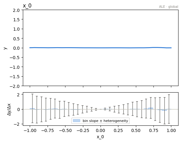
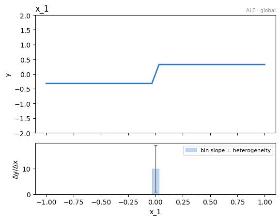
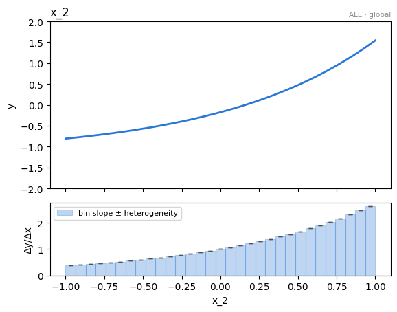
    ale.plot(feature=feature, centering=True, heterogeneity=True, y_limits=[-2, 2])

ALE states that:

• Feature \(x_1\):
  The heterogeneity varies across all values of \(x_1\). It starts large at \(x_1 = -1\), decreases until it becomes zero at \(x_1 = 0\), and then increases again until \(x_1 = 1\).
  This behavior contrasts with the heterogeneity observed in the PDP, which has two zero-points at \(x_1 = \pm \frac{2}{3}\).

• Feature \(x_2\):
  Heterogeneity is observed only around \(x_2 = 0\). This behavior also contrasts PDP's heterogeneity which is constant for all values of \(x_2\)

• Feature \(x_3\):
  No heterogeneity is present for this feature.

Derivations

For x_1:

The \(x_1\)-axis is divided into \(K\) equal bins, indexed by \(k = 1, \ldots, K\), with the center of the \(k\)-th bin denoted as \(c_k\). In each bin: if \(x_2 < 0\), the local effects is \(-2c_k\), and if \(x_2 \geq 0\) the local effect is \(2 c_k\). This gives a variance of \(4c_k^2\) within each bin. Therefore, \(h(x_1) = 4c_k^2\) where \(k\) is the index of the bin that contains \(x_1\).

\[\begin{align} h(x_1) &= \frac{1}{|\mathcal{S}_k|} \sum_{\mathbf{x}^i \in \mathcal{S}_k} \left ( \frac{f(z_k, x_2^i, x_3^i) - f(z_{k-1}, x_2^i, x_3^i)}{z_k - z_{k-1}} - \hat{\mu}_k^{ALE} \right )^2 \\ &= \frac{1}{|\mathcal{S}_k|} \sum_{\mathbf{x}^i \in \mathcal{S}_k} \left ( \frac{-2c_k(z_k - z_{k-1}) \mathbb{1}_{x_2^i < 0} + 2c_k(z_k - z_{k-1}) \mathbb{1}_{x_2^i \geq 0}}{z_k - z_{k-1}} \right )^2 \\ &= \frac{1}{|\mathcal{S}_k|} \sum_{\mathbf{x}^i \in \mathcal{S}_k} 4 c_k^2 \\ &= 4 c_k^2 \end{align}\]

For \(x_2\):

In all bins except the central one, the local effects are zero. In the central bin, however, the local effects are $ 2(x_1^i)^2 $, which introduces some heterogeneity. So, if $ x_2 $ is not in the central bin $ k = K/2 $, \(h(x_2) = 0\). If $ x_2 $ is in the central bin $ k = K/2 $:

\[\begin{align} h(x_2) &= \frac{1}{|\mathcal{S}_k|} \sum_{\mathbf{x}^i \in \mathcal{S}_k} \left( \frac{f(z_k, x_2^i, x_3^i) - f(z_{k-1}, x_2^i, x_3^i)}{z_k - z_{k-1}} - \hat{\mu}_k^{ALE} \right)^2 \\ &= \frac{2}{z_k - z_{k-1}} \frac{1}{|\mathcal{S}_k|} \sum_{\mathbf{x}^i \in \mathcal{S}_k} (x_1^i)^2 \\ &= \frac{2}{3}(z_k - z_{k-1}) \\ &\approx 10 \text{ for } K=31 \end{align}\]

So: \begin{align} h(x_2) &= \begin{cases} 0, & \text{if } x_2 \text{ is not in the central bin (}\ k = K/2\text{)}, \ \frac{31}{3} \approx 10 & \text{if } x_2 \text{ is in the central bin (}\ k = K/2\text{)}. \end{cases} \ \end{align}

For \(x_3\):

The effect is zero everywehere.

# The closed form below lives in `effector.benchmarks` — the SAME function the
# test suite asserts against (tests/test_functional_conditional_interaction.py),
# so this notebook and the tests can never disagree about the right answer.
ale_ground_truth = bench.ale_bin_variance_gt

# make a test
K = 31
bin_centers = np.linspace(-1 + 1/K, 1 - 1/K, K)
for feature in [0, 1, 2]:
    bin_var = ale.payload(feature)["bin_variance"]
    gt_var = ale_ground_truth(feature)
    mask = ~np.isnan(gt_var)
    np.testing.assert_allclose(bin_var[mask], gt_var[mask], atol=1e-1)

Conclusions

Is the heterogeneity implied by the ALE plots meaningful? It is

RHALE

Effector

Let's see below the RHALE effects for each feature, using effector.

rhale = effector.RHALE(x, model.predict, model.jacobian, axis_limits=dataset.axis_limits)
rhale.fit(features="all", centering=True, binning_method=effector.axis_partitioning.Fixed(nof_bins=31))

for feature in [0, 1, 2]:
    rhale.plot(feature=feature, centering=True, heterogeneity=True, y_limits=[-2, 2])

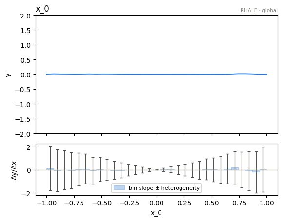
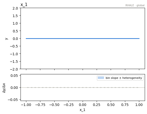
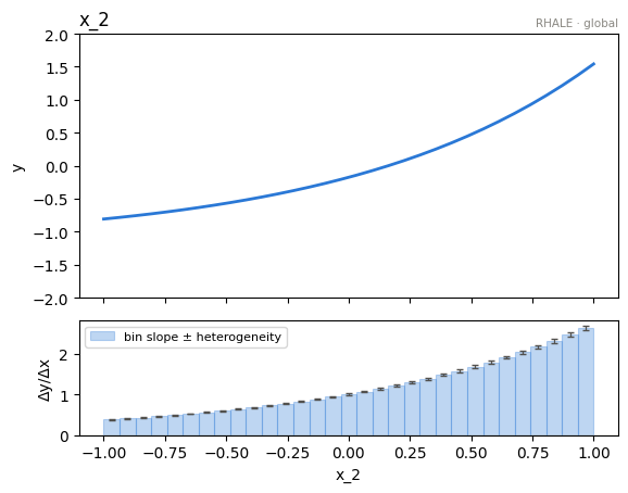
RHALE states that:

• Feature \(x_1\): As in ALE, the heterogeneity varies across all values of \(x_1\). It starts large at \(x_1 = -1\), decreases until it becomes zero at \(x_1 = 0\), and then increases again until \(x_1 = 1\).

• Feature \(x_2\):
  No heterogeneity is present for this feature.

• Feature \(x_3\):
  No heterogeneity is present for this feature.

Derivations

For \(x_1\): within a bin centered at \(c_k\), the derivatives are \(\frac{\partial f}{\partial x_1} = -2x_1 \mathbb{1}_{x_2<0} + 2x_1 \mathbb{1}_{x_2 \geq 0}\), i.e. \(\pm 2 x_1\) with equal probability, so their per-bin variance is

\[H_k(x_1) = \mathbb{E}[(\pm 2 c_k)^2] - \underbrace{\mathbb{E}[\pm 2 c_k]^2}_{=0} = 4 c_k^2.\]

For \(x_2\): \(\frac{\partial f}{\partial x_2} = 0\) almost everywhere, so every bin has zero variance:

\[H_k(x_2) = 0.\]

Note the contrast with ALE: the ALE bin containing \(x_2 = 0\) shows a large variance spike (the finite differences straddle the jump), while the derivative never sees the jump at all.

For \(x_3\): \(\frac{\partial f}{\partial x_3} = e^{x_3}\) is deterministic — all instances in a bin have (nearly) the same derivative, so

\[H_k(x_3) \approx 0.\]

Tests

# make a test
for feature in [0, 1, 2]:
    bin_var = rhale.payload(feature)["bin_variance"]
    gt_var = bench.rhale_bin_variance_gt(feature)
    np.testing.assert_allclose(bin_var, gt_var, atol=1e-1)

Conclusions

RHALE agrees with ALE on where the heterogeneity is (\(x_1\)) and where it is not (\(x_3\)), and it is cleaner on \(x_2\): the ALE spike at the jump bin is an artifact of finite differences straddling the discontinuity, whereas the derivative-based RHALE correctly reports zero heterogeneity everywhere.

Cross-method sanity check

The one-liner effector.explain with every engine this notebook's model supports. Everything must run end to end; the closing table puts the reads side by side. Where methods disagree — ranking, accepted splits, R² — that is a property of the data/model worth a closer look, not an error.

from pathlib import Path
_out = Path("reports") / "05_conditional_interaction_independent_uniform_heter"
_out.mkdir(parents=True, exist_ok=True)

# === cross-method sweep: effector.explain on every applicable engine ======
sweep_reports = {}
for _m in ["pdp", "derpdp", "ale", "rhale", "shapdp"]:
    _kw = {"nof_instances": 300} if _m == "shapdp" else {}
    print(f"--- {_m} " + "-" * 50)
    sweep_reports[_m] = effector.explain(
        x, model.predict, model.jacobian, method=_m, **_kw
    )
    if _m != "pdp":  # the published report is the narrated one above
        sweep_reports[_m].to_html(_out / f"report_{_m}.html")

print()
print(f"{'method':<8} {'ranking (plotted)':<44} {'GAM R2':>8} {'final R2':>9}  splits")
for _m, _r in sweep_reports.items():
    _rank = " > ".join(fr.name for fr in _r.features)
    _ev = _r.explained_variance
    if _ev:
        _sp = "; ".join(f"{s['name']} on {s['on']}" for s in _ev["stages"]) or "none"
        print(f"{_m:<8} {_rank:<44} {_ev['gam_r2']:>7.1%} {_ev['regional_r2']:>8.1%}  {_sp}")
    else:
        print(f"{_m:<8} {_rank:<44} {'-':>7} {'-':>8}  (derivative scale: no variance ledger)")

print(f"\nreports stored in {_out}/")

--- pdp --------------------------------------------------


[effector] global effects   (GAM)  -> 85.8% of the model's variance
           regional effects (CALM) -> 99.8%
--- derpdp --------------------------------------------------


/home/givasile/github/packages/effector/effector/report.py:606: UserWarning: This figure includes Axes that are not compatible with tight_layout, so results might be incorrect.
  fig.tight_layout()


--- ale --------------------------------------------------


[effector] global effects   (GAM)  -> 84.8% of the model's variance
           regional effects (CALM) -> 98.9%


/home/givasile/github/packages/effector/effector/report.py:606: UserWarning: This figure includes Axes that are not compatible with tight_layout, so results might be incorrect.
  fig.tight_layout()


--- rhale --------------------------------------------------


[effector] global effects   (GAM)  -> 68.6% of the model's variance
           regional effects (CALM) -> 100.0%


/home/givasile/github/packages/effector/effector/report.py:606: UserWarning: This figure includes Axes that are not compatible with tight_layout, so results might be incorrect.
  fig.tight_layout()


--- shapdp --------------------------------------------------


[effector] global effects   (GAM)  -> 82.2% of the model's variance
           regional effects (CALM) -> 97.8%


/home/givasile/github/packages/effector/effector/report.py:606: UserWarning: This figure includes Axes that are not compatible with tight_layout, so results might be incorrect.
  fig.tight_layout()



method   ranking (plotted)                              GAM R2  final R2  splits
pdp      x_2 > x_1 > x_0                                85.8%    99.8%  x_0 on x_1
derpdp   x_2                                                -        -  (derivative scale: no variance ledger)
ale      x_2 > x_1 > x_0                                84.8%    98.9%  x_0 on x_1
rhale    x_2 > x_0                                      68.6%   100.0%  x_0 on x_1
shapdp   x_2 > x_1 > x_0                                82.2%    97.8%  x_1 on x_0; x_0 on x_1

reports stored in reports/05_conditional_interaction_independent_uniform_heter/