Model with general interaction

• Author: givasile
• Runtime: ~5 s
• Description: Global effects and heterogeneity (PDP, ALE, RHALE) on a model with a general-form interaction \(x_1 x_2^2\); all estimates are derived analytically and tested against effector.benchmarks.
• 📄 The whole notebook in one page: PDP report

In this example, we show global effects of a model with general form interactions using PDP, ALE, and RHALE. In particular, we:

1. show how to use effector to estimate the global effects using PDP, ALE, and RHALE
2. provide the analytical formulas for the global effects
3. test that (1) and (2) match

We will use the following function:

\[ f(x_1, x_2, x_3) = x_1 x_2^2 + e^{x_3} \]

where the features \(x_1\), \(x_2\), and \(x_3\) are independent and uniformly distributed in the interval \([-1, 1]\).

The model contains an interaction between \(x_1\) and \(x_2\) caused by the term:

\[ f_{1,2}(x_1, x_2) = x_1 x_2^2. \]

This means that the effect of \(x_1\) on the output depends on the value of \(x_2\), and vice versa. Consequently, there is no universally agreed-upon way to separate the effect of \(f_{1,2}\) into two components: one that corresponds solely to \(x_1\) and one solely to \(x_2\). Different global effect methods (such as PDP, ALE, and RHALE) adopt different strategies to handle this interaction.

In contrast, \(x_3\) does not interact with any other feature, so its effect can be easily computed as \(e^{x_3}\).

import numpy as np
import matplotlib.pyplot as plt
import effector

np.random.seed(21)

bench = effector.benchmarks.GeneralInteractionUniform()
model = bench.model
dataset = bench.dataset
x = bench.generate_data(1_000)

PDP

Effector

Let's see below the PDP effects for each feature, using effector.

pdp = effector.PDP(x, model.predict, axis_limits=dataset.axis_limits)
pdp.fit(features="all", centering=True)
for feature in [0, 1, 2]:
    pdp.plot(feature=feature, centering=True, y_limits=[-2, 2], heterogeneity=False)

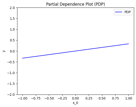
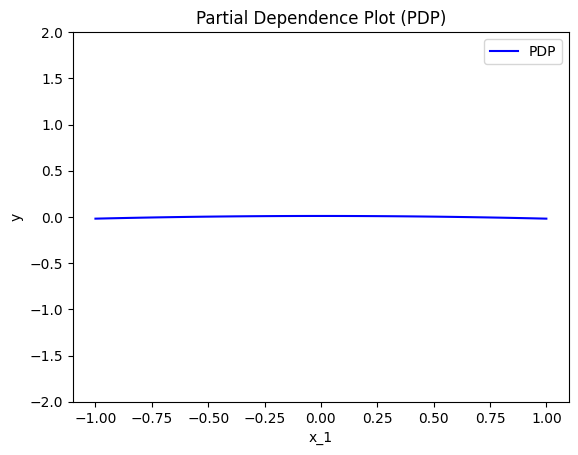
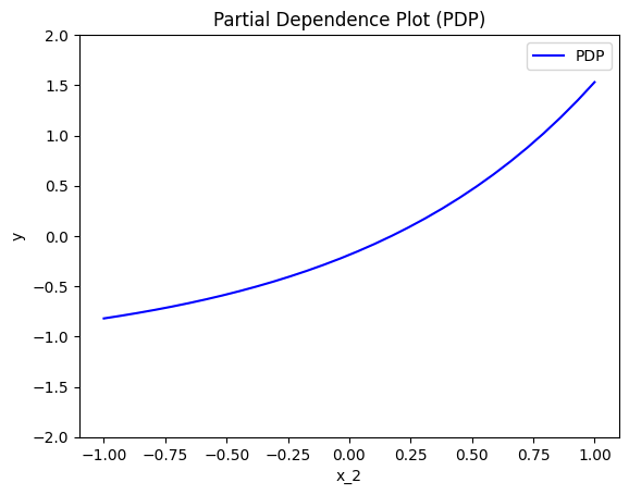
PDP states that:

• \(x_1\) has an average effect proportional to \(\frac{1}{3} x_1\) on the model output.
• \(x_2\) has a constant effect on the model output due to \(x_2^2\), which is symmetric about \(x_2 = 0\).
• \(x_3\) has an effect of \(e^{x_3}\).

Derivations

How PDP leads to these explanations? Are they meaningfull? Let's have some analytical derivations. If you don't care about the derivations, skip the following three cells and go directly to the coclusions.

For \(x_1\):

\[\begin{align} PDP(x_1) &\propto \frac{1}{N} \sum_{i=1}^{N} f(x_1, \mathbf{x}^i_{/1}) \\ &\propto \frac{1}{N} \sum_{i=1}^{N} \left( x_1 x_2^{i,2} + e^{x_3^i} \right) \\ &\propto x_1 \cdot \frac{1}{N} \sum_{i=1}^{N} x_2^{i,2} + \frac{1}{N} \sum_{i=1}^{N} e^{x_3^i} \\ &\propto x_1 \cdot \mathbb{E}[x_2^2] + c, \end{align}\]

where \(\mathbb{E}[x_2^2] = \frac{1}{3}\) for \(x_2 \sim \mathcal{U}(-1, 1)\) and \(c\) is the constant contribution from \(e^{x_3}\). Therefore:

\[ PDP(x_1) = \frac{1}{3} x_1 + c. \]

For \(x_2\):

\[\begin{align} PDP(x_2) &\propto \frac{1}{N} \sum_{i=1}^{N} f(x_2, \mathbf{x}_{/2}^i) \\ &\propto \frac{1}{N} \sum_{i=1}^{N} \left( x_1^i (x_2)^2 + e^{x_3^i} \right) \\ &\propto \left( x_2^2 \cdot \frac{1}{N} \sum_{i=1}^{N} x_1^i \right) + \frac{1}{N} \sum_{i=1}^{N} e^{x_3^i}. \end{align}\]

Since \(\frac{1}{N} \sum_{i=1}^{N} x_1^i = 0\) for \(x_1 \sim \mathcal{U}(-1, 1)\): $$ PDP(x_2) \propto \mathbb{E}[e^{x_3}]. $$

Thus: $$ PDP(x_2) = c, $$

where \(c\) is the constant contribution from \(e^{x_3}\).

For \(x_3\):

\[\begin{align} PDP(x_3) &\propto \frac{1}{N} \sum_{i=1}^{N} f(x_3, \mathbf{x}_{/3}^i) \\ &\propto \frac{1}{N} \sum_{i=1}^{N} \left( x_1^i (x_2^i)^2 + e^{x_3} \right) \\ &\propto \frac{1}{N} \sum_{i=1}^{N} x_1^i (x_2^i)^2 + e^{x_3}. \end{align}\]

Since \(\frac{1}{N} \sum_{i=1}^{N} x_1^i (x_2^i)^2 = 0\) (as \(x_1\) and \((x_2^i)^2\) are independent, and \(\mathbb{E}[x_1] = 0\)): $$ PDP(x_3) \propto e^{x_3}. $$

Thus: $$ PDP(x_3) = e^{x_3}. $$

Conclusions

Are the PDP effects intuitive?

• For \(x_1\), the effect is proportional to \(\frac{1}{3} x_1\). The term \(x_1 x_2^2\) involves an interaction with \(x_2\), but since \(x_2^2 \sim \mathcal{U}([0,1])\), the interaction averages out uniformly, leaving a proportional effect of \(\frac{1}{3} x_1\).
• For \(x_2\), the effect is constant because \(x_2^2\) is symmetric about \(x_2 = 0\). Since \(x_2^2\) contributes positively and does not depend on the sign of \(x_2\), the PDP reflects only the additive constant contribution from \(e^{x_3}\).
• For \(x_3\), the effect is \(e^{x_3}\), as expected, since this term directly corresponds to \(x_3\) and has no interaction with other variables.

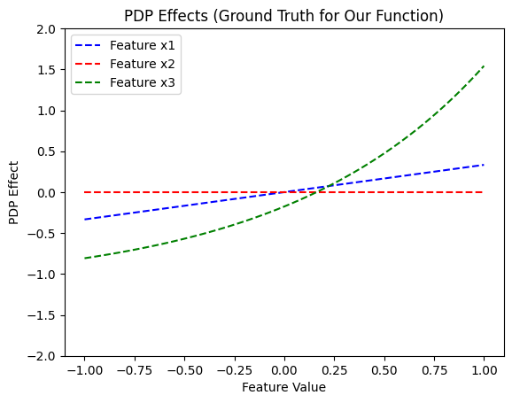
Tests

# The closed form below lives in `effector.benchmarks` — the SAME function the
# test suite asserts against (tests/test_functional_general_interaction.py),
# so this notebook and the tests can never disagree about the right answer.
pdp_ground_truth = bench.pdp_gt

xx = np.linspace(-1, 1, 100)
y_pdp = []

for feature in [0, 1, 2]:
    y_pdp.append(pdp_ground_truth(feature, xx))

plt.figure()
plt.title("PDP Effects (Ground Truth for Our Function)")
color_palette = ["blue", "red", "green"]
feature_labels = ["Feature x1", "Feature x2", "Feature x3"]
for feature in [0, 1, 2]:
    plt.plot(
        xx,
        y_pdp[feature],
        color=color_palette[feature],
        linestyle="--",
        label=feature_labels[feature],
    )

plt.legend()
plt.xlim([-1.1, 1.1])
plt.ylim([-2, 2])
plt.xlabel("Feature Value")
plt.ylabel("PDP Effect")
plt.show()

# make a test
xx = np.linspace(-1, 1, 100)
for feature in [0, 1, 2]:
    y_pdp = pdp.eval(feature=feature, xs=xx, centering=True)
    y_gt = pdp_ground_truth(feature, xx)
    np.testing.assert_allclose(y_pdp, y_gt, atol=1e-1)

ALE

Effector

Let's see below the PDP effects for each feature, using effector.

ale = effector.ALE(x, model.predict, axis_limits=dataset.axis_limits)
ale.fit(features="all", centering=True, binning_method=effector.axis_partitioning.Fixed(nof_bins=31))

for feature in [0, 1, 2]:
    ale.plot(feature=feature, centering=True, y_limits=[-2, 2], heterogeneity=False)

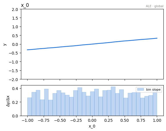
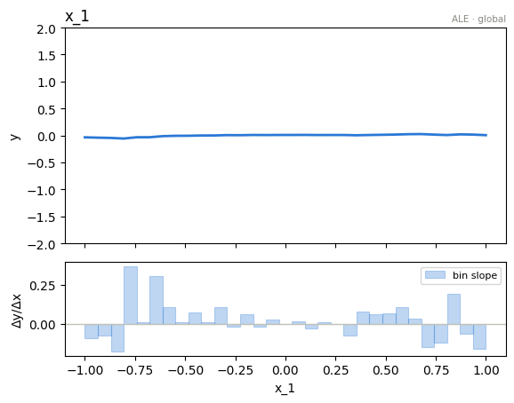
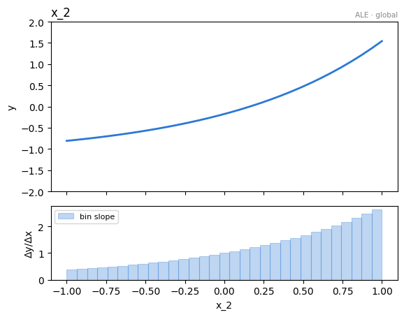
ALE states that:

• For \(x_1\): The ALE effect is proportional to \(\frac{1}{3} x_1\). This reflects the linear relationship between \(x_1\) and the model output, averaged over the distribution of \(x_2\). The result aligns with the PDP, as the average effect of \(x_2^2\) on \(x_1\) remains consistent.

• For \(x_2\): The ALE effect is constant, as \(x_2^2\) contributes symmetrically to the model output. This results in no variation with \(x_2\), and the effect is consistent with the PDP. The interaction terms cancel out on average, leaving only the baseline constant.

• For \(x_3\): The ALE effect is \(e^{x_3}\), reflecting the direct contribution of the exponential term \(e^{x_3}\) in the model. This is identical to the PDP effect since \(x_3\) does not interact with other features.

Derivations

\[\begin{align} ALE(x_1) &\propto \sum_{k=1}^{k_{x_1}} \frac{1}{| \mathcal{S}_k |} \sum_{i: x^i \in \mathcal{S}_k} \left[ f(z_k, x^i_2, x^i_3) - f(z_{k-1}, x^i_2, x^i_3) \right] \\ &\propto \sum_{k=1}^{k_{x_1}} \frac{1}{| \mathcal{S}_k |} \sum_{i: x^i \in \mathcal{S}_k} \left[ z_k x_2^{i,2} + e^{x_3^i} - (z_{k-1} x_2^{i,2} + e^{x_3^i}) \right] \\ &\propto \sum_{k=1}^{k_{x_1}} \frac{1}{| \mathcal{S}_k |} \sum_{i: x^i \in \mathcal{S}_k} \left[ (z_k - z_{k-1}) x_2^{i,2} \right]. \end{align}\]

Since \(x_2^{i,2} \sim \mathcal{U}([0, 1])\), its expected value is:

\[\begin{align} \mathbb{E}[x_2^2] &= \frac{1}{3}. \end{align}\]

Thus:

\[\begin{align} ALE(x_1) &\propto (z_k - z_{k-1}) \cdot \mathbb{E}[x_2^2] \\ &= \frac{1}{3} x_1. \end{align}\]

\[\begin{align} ALE(x_2) &\propto \sum_{k=1}^{k_{x_2}} \frac{1}{| \mathcal{S}_k |} \sum_{i: x^i \in \mathcal{S}_k} \left[ f(x^i_1, z_k, x^i_3) - f(x^i_1, z_{k-1}, x^i_3) \right] \\ &\propto \sum_{k=1}^{k_{x_2}} \frac{1}{| \mathcal{S}_k |} \sum_{i: x^i \in \mathcal{S}_k} \left[ x_1^i z_k^2 + e^{x_3^i} - (x_1^i z_{k-1}^2 + e^{x_3^i}) \right] \\ &\propto \sum_{k=1}^{k_{x_2}} \frac{1}{| \mathcal{S}_k |} \sum_{i: x^i \in \mathcal{S}_k} \left[ x_1^i (z_k^2 - z_{k-1}^2) \right]. \end{align}\]

Since \(x_1^i \sim \mathcal{U}(-1, 1)\), its expected value is zero:

\[\begin{align} \mathbb{E}[x_1] &= 0. \end{align}\]

Thus:

\[\begin{align} ALE(x_2) &\propto 0. \end{align}\]

\[\begin{align} ALE(x_3) &\propto \sum_{k=1}^{k_{x_3}} \frac{1}{| \mathcal{S}_k |} \sum_{i: x^{(i)} \in \mathcal{S}_k} \left [ f(x^i_1, x^i_2, z_k) - f(x^i_1, x^i_2, z_{k-1}) \right ] \\ &\propto \sum_{k=1}^{k_{x_3}} \frac{1}{| \mathcal{S}_k |} \sum_{i: x^{(i)} \in \mathcal{S}_k} \left [ e^{z_k} - e^{z_{k-1}} \right ] \\ &\approx e^{x_3} \end{align}\]

Tests

# The closed form below lives in `effector.benchmarks` — the SAME function the
# test suite asserts against (tests/test_functional_general_interaction.py),
# so this notebook and the tests can never disagree about the right answer.
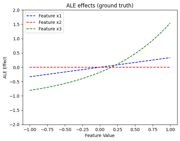
ale_ground_truth = bench.ale_gt

xx = np.linspace(-1, 1, 100)
y_ale = []
for feature in [0, 1, 2]:
    y_ale.append(ale_ground_truth(feature, xx))

plt.figure()
plt.title("ALE effects (ground truth)")
color_pallette = ["blue", "red", "green"]
feature_labels = ["Feature x1", "Feature x2", "Feature x3"]
for feature in [0, 1, 2]:
    plt.plot(
        xx, 
        y_ale[feature], 
        color=color_pallette[feature], 
        linestyle="--",
        label=feature_labels[feature]
    )
plt.legend()
plt.xlim([-1.1, 1.1])
plt.ylim([-2, 2])
plt.xlabel("Feature Value")
plt.ylabel("ALE Effect")
plt.show()

xx = np.linspace(-1, 1, 100)
for feature in [0, 1, 2]:
    y_ale = ale.eval(feature=feature, xs=xx, centering=True)
    y_gt = ale_ground_truth(feature, xx)

    # hack to remove the effect at undefined region
    if feature == 1:
        K = 31
        ind = np.logical_and(xx > -1/K, xx < 1/K)
        y_ale[ind] = 0
        y_gt[ind] = 0

    np.testing.assert_allclose(y_ale, y_gt, atol=1e-1)

Conclusions

Are the ALE effects intuitive?

ALE effects are identical to PDP effects which, as discussed above, can be considered intutive.

RHALE

Effector

Let's see below the RHALE effects for each feature, using effector.

rhale = effector.RHALE(x, model.predict, model.jacobian, axis_limits=dataset.axis_limits)
rhale.fit(features="all", centering=True)

for feature in [0, 1, 2]:
    rhale.plot(feature=feature, centering=True, y_limits=[-2, 2], heterogeneity=False)

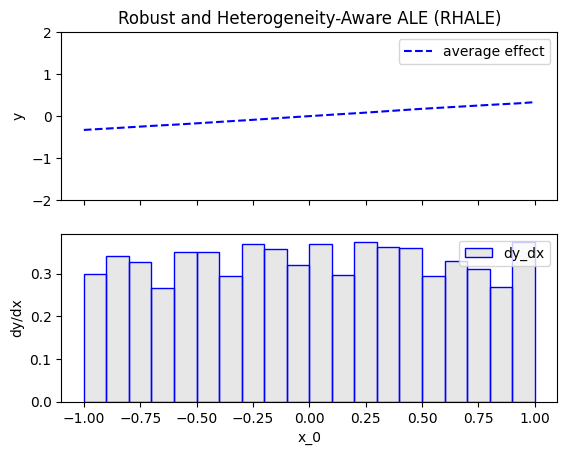
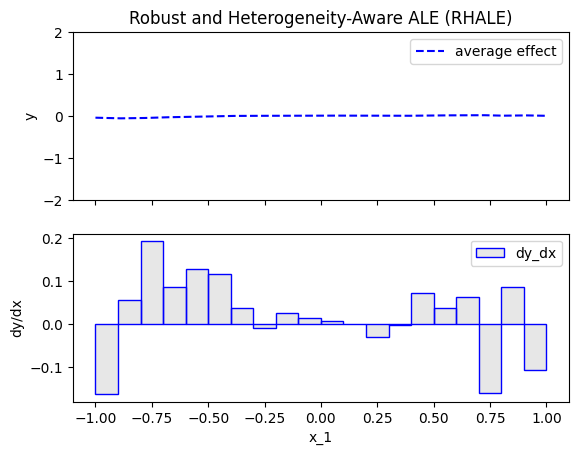
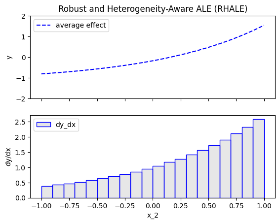
RHALE states that:

• \(x_1\) has an average effect proportional to \(\frac{1}{3} x_1\) (same as PDP and ALE)
• \(x_2\) has a zero average effect: \(\mathbb{E}[x_1] = 0\), so the interaction term \(x_1 x_2^2\) vanishes on average (same as PDP and ALE)
• \(x_3\) has an effect of \(e^{x_3}\) (same as PDP and ALE)

For this model — smooth, with independent features — all three methods agree everywhere; the differences between them only appear under discontinuities (notebook 05) or correlated features (notebook 02).

Derivations

\[\begin{align} RHALE(x_1) &\propto \sum_{k=1}^{k_{x_1}} \frac{1}{| \mathcal{S}_k |} (z_k - z_{k-1}) \sum_{i: x^i \in \mathcal{S}_k} \left[ \frac{\partial f}{\partial x_1}(\mathbf{x}^i) \right] \\ &\propto \sum_{k=1}^{k_{x_1}} \frac{1}{| \mathcal{S}_k |} (z_k - z_{k-1}) \sum_{i: x^i \in \mathcal{S}_k} \left[ x_2^{i,2} \right]. \end{align}\]

Since \(x_2^{i,2} \sim \mathcal{U}([0, 1])\), its expected value is:

\[\begin{align} \mathbb{E}[x_2^2] &= \frac{1}{3}. \end{align}\]

Thus:

\[\begin{align} RHALE(x_1) &\propto (z_k - z_{k-1}) \cdot \mathbb{E}[x_2^2] \\ &= \frac{1}{3} x_1. \end{align}\]

\[\begin{align} RHALE(x_2) &\propto \sum_{k=1}^{k_{x_2}} \frac{1}{| \mathcal{S}_k |} (z_k - z_{k-1}) \sum_{i: x^i \in \mathcal{S}_k} \left[ \frac{\partial f}{\partial x_2}(\mathbf{x}^i) \right] \\ &\propto \sum_{k=1}^{k_{x_2}} \frac{1}{| \mathcal{S}_k |} (z_k - z_{k-1}) \sum_{i: x^i \in \mathcal{S}_k} \left[ 2 x_1^i x_2^i \right]. \end{align}\]

Since \(x_1^i \sim \mathcal{U}(-1, 1)\) and \(x_2^i \sim \mathcal{U}(-1, 1)\), their expected product is:

\[\begin{align} \mathbb{E}[x_1 x_2] &= 0. \end{align}\]

Thus:

\[\begin{align} RHALE(x_2) &\propto 0. \end{align}\]

\[\begin{align} RHALE(x_3) &\propto \sum_{k=1}^{k_{x_3}} \frac{1}{| \mathcal{S}_k |} (z_k - z_{k-1}) \sum_{i: x^i \in \mathcal{S}_k} \left [ \frac{\partial f}{\partial x_3}(\mathbf{x}^i) \right ] \\ &\propto \sum_{k=1}^{k_{x_3}} \frac{1}{| \mathcal{S}_k |} (z_k - z_{k-1}) \sum_{i: x^i \in \mathcal{S}_k} \left [ e^{x_3} \right ] \\ &\approx e^{x_3} \end{align}\]

Tests

# The closed form below lives in `effector.benchmarks` — the SAME function the
# test suite asserts against (tests/test_functional_general_interaction.py),
# so this notebook and the tests can never disagree about the right answer.
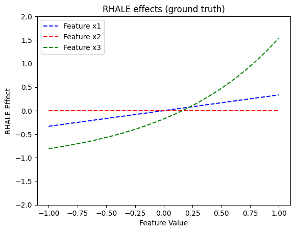
rhale_ground_truth = bench.rhale_gt

xx = np.linspace(-1, 1, 100)
y_rhale = []
for feature in [0, 1, 2]:
    y_rhale.append(rhale_ground_truth(feature, xx))

plt.figure()
plt.title("RHALE effects (ground truth)")
color_pallette = ["blue", "red", "green"]
feature_labels = ["Feature x1", "Feature x2", "Feature x3"]
for feature in [0, 1, 2]:
    plt.plot(
        xx, 
        y_rhale[feature], 
        color=color_pallette[feature], 
        linestyle= "--",
        label=feature_labels[feature]
    )
plt.legend()
plt.xlim([-1.1, 1.1])
plt.ylim([-2, 2])
plt.xlabel("Feature Value")
plt.ylabel("RHALE Effect")
plt.show()

for feature in [0, 1, 2]:
    y_ale = rhale.eval(feature=feature, xs=xx, centering=True)
    y_gt = rhale_ground_truth(feature, xx)
    np.testing.assert_allclose(y_ale, y_gt, atol=1e-1)

Conclusions

Are the RHALE effects intuitive?

Since \(f(x_1, x_2, x_3)\) is smooth and differentiable with respect to all features, RHALE behaves consistently with ALE and PDP for all features. It correctly captures the linear effect of \(x_1\), the symmetric constant contribution of \(x_2^2\) as zero, and the exponential effect of \(x_3\).

Heterogeneity

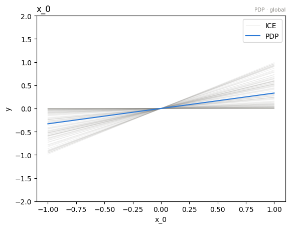
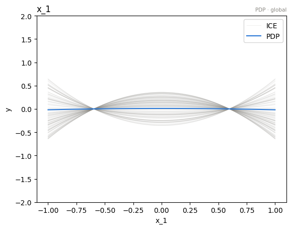
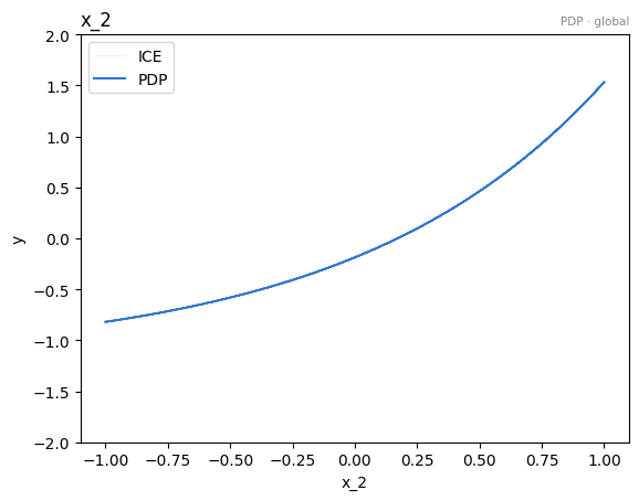
The mean effects hide the most interesting property of this model: the interaction \(x_1 x_2^2\) is invisible in the mean effect of \(x_2\) (because \(\mathbb{E}[x_1] = 0\)) but fully visible in its heterogeneity — the variance of the (centered) ICE curves.

For \(x_1\): the centered ICE at position \(x_1\) is \(x_1 (x_{2,i}^2 - \text{const})\), so its variance across instances is

\[h(x_1) = x_1^2 \, \mathrm{Var}[x_2^2] = \frac{4}{45} x_1^2.\]

For \(x_2\): the centered ICE is \(x_{1,i}(x_2^2 - \mathbb{E}[x_2^2])\), so

\[h(x_2) = \left(x_2^2 - \tfrac{1}{3}\right)^2 \mathbb{E}[x_1^2] = \frac{(x_2^2 - 1/3)^2}{3}.\]

For \(x_3\): the additive \(e^{x_3}\) term is the same for every instance, so \(h(x_3) = 0\).

pdp = effector.PDP(x, model.predict, axis_limits=dataset.axis_limits, nof_instances="all")
for feature in [0, 1, 2]:
    pdp.plot(feature=feature, centering=True, heterogeneity="ice", y_limits=[-2, 2])

Tests

# make a test
xx = np.linspace(-1, 1, 100)
for feature in [0, 1, 2]:
    pdp_heter = pdp.eval_heter(feature=feature, xs=xx)
    np.testing.assert_allclose(pdp_heter, bench.pdp_heter_gt(feature, xx), atol=1e-1)

Conclusions

\(x_2\) is the textbook case for why heterogeneity matters: its mean effect is exactly zero, yet the ICE curves fan out with variance \((x_2^2 - 1/3)^2 / 3\) — an interaction that a mean-only reading would miss entirely. This is also the signal that regional methods exploit to find meaningful subspaces.

Importance & one-click explanation

Two conveniences on top of the global effects above:

• importances() ranks features by the dispersion of the mean effect — the \(\mu\)-twin of heterogeneity. Here \(x_3\) (the \(e^{x_3}\) term) and \(x_1\) (the \(\tfrac{1}{3}x_1\) slope) carry the visible mean effect, while \(x_2\) has a mean effect of ~0 and so scores near zero — even though it is the most heterogeneous feature.
• effector.explain(...) runs the whole pipeline once (fit → rank → per-feature mean/heterogeneity curves → region search) and returns a serializable Report with a self-contained HTML view.

# per-feature importance = dispersion of the mean effect (mu-twin of heterogeneity)
print("importances:", np.round(pdp.importances(), 3))

# one-click auto-explanation -> Report (serializable; self-contained HTML)
report = effector.explain(x, model.predict, method="pdp", nof_instances="all")
report.show()

# the whole notebook, in one page: the report published with this example
from pathlib import Path
_out = Path("reports") / "06_general_interaction_independent_uniform_global"
_out.mkdir(parents=True, exist_ok=True)
report.to_html(_out / "report_pdp.html")

importances: [0.19  0.009 0.668]
[effector] global effects   (GAM)  -> 94.0% of the model's variance
           regional effects (CALM) -> 99.6%

  ════════════════════════════════════════════════════════════════════════
  PDP report  ·  target: y
  ════════════════════════════════════════════════════════════════════════

  DATA & MODEL
  ────────────────────────────────────────────────────────────────────────
    instances     1,000
    features      3  ·  3 continuous
    model output  mean 1.17 · std 0.7 · range [-0.432, 3.1]

  EXPLAINED VARIANCE
  ────────────────────────────────────────────────────────────────────────
    step         split on                 solo     ΔR²      R²       heter
    ──────────────────────────────────────────────────────────────────────
    GAM          (all features global)       —       —   94.0%           —
  + x_1          x_0                     +5.6%   +5.6%   99.6% 0.17 → 0.04
    ──────────────────────────────────────────────────────────────────────
    FINAL                                                99.6%

  REJECTED SPLITS                                            min gain 1.0%
  ────────────────────────────────────────────────────────────────────────
    feature      split on                 solo     ΔR²    reason
    ──────────────────────────────────────────────────────────────────────
  ✗ x_0          x_1                     +4.8%   -4.0%    redundant

    ✗ redundant: it would explain variance on its own (see solo),
      but the accepted splits already account for it.

  FEATURES                                ranked, in the selected snapshot
  ────────────────────────────────────────────────────────────────────────
    feature        importance                          heter      #regions
    ──────────────────────────────────────────────────────────────────────
    x_2                0.6679  ██████████████████     0.0000             1
    x_0                0.1897  █████                  0.1713             1
    x_1                0.1481  ████                   0.0440             4
    ──────────────────────────────────────────────────────────────────────
    the features above carry 100% of the total importance mass



Feature 1 - Full partition tree:
🌳 Full Tree Structure:
───────────────────────
x_1 🔹 [id: 0 | heter: 0.17 | inst: 1000 | w: 1.00]
    x_0 < -0.00 🔹 [id: 1 | heter: 0.09 | inst: 510 | w: 0.51]
        x_0 < -0.50 🔹 [id: 2 | heter: 0.04 | inst: 268 | w: 0.27]
        -0.50 ≤ x_0 < -0.00 🔹 [id: 3 | heter: 0.05 | inst: 242 | w: 0.24]
    x_0 ≥ -0.00 🔹 [id: 4 | heter: 0.09 | inst: 490 | w: 0.49]
        -0.00 ≤ x_0 < 0.50 🔹 [id: 5 | heter: 0.04 | inst: 254 | w: 0.25]
        x_0 ≥ 0.50 🔹 [id: 6 | heter: 0.04 | inst: 236 | w: 0.24]
--------------------------------------------------
Feature 1 - Statistics per tree level:
🌳 Tree Summary:
─────────────────
Level 0🔹heter: 0.17
    Level 1🔹heter: 0.09 | 🔻0.09 (50.14%)
        Level 2🔹heter: 0.04 | 🔻0.04 (48.85%)




/home/givasile/github/packages/effector/effector/report.py:606: UserWarning: This figure includes Axes that are not compatible with tight_layout, so results might be incorrect.
  fig.tight_layout()

Cross-method sanity check

The one-liner effector.explain with every engine this notebook's model supports. Everything must run end to end; the closing table puts the reads side by side. Where methods disagree — ranking, accepted splits, R² — that is a property of the data/model worth a closer look, not an error.

from pathlib import Path
_out = Path("reports") / "06_general_interaction_independent_uniform_global"
_out.mkdir(parents=True, exist_ok=True)

# === cross-method sweep: effector.explain on every applicable engine ======
sweep_reports = {}
for _m in ["pdp", "derpdp", "ale", "rhale", "shapdp"]:
    _kw = {"nof_instances": 300} if _m == "shapdp" else {}
    print(f"--- {_m} " + "-" * 50)
    sweep_reports[_m] = effector.explain(
        x, model.predict, model.jacobian, method=_m, **_kw
    )
    if _m != "pdp":  # the published report is the narrated one above
        sweep_reports[_m].to_html(_out / f"report_{_m}.html")

print()
print(f"{'method':<8} {'ranking (plotted)':<44} {'GAM R2':>8} {'final R2':>9}  splits")
for _m, _r in sweep_reports.items():
    _rank = " > ".join(fr.name for fr in _r.features)
    _ev = _r.explained_variance
    if _ev:
        _sp = "; ".join(f"{s['name']} on {s['on']}" for s in _ev["stages"]) or "none"
        print(f"{_m:<8} {_rank:<44} {_ev['gam_r2']:>7.1%} {_ev['regional_r2']:>8.1%}  {_sp}")
    else:
        print(f"{_m:<8} {_rank:<44} {'-':>7} {'-':>8}  (derivative scale: no variance ledger)")

print(f"\nreports stored in {_out}/")

--- pdp --------------------------------------------------
[effector] global effects   (GAM)  -> 94.0% of the model's variance
           regional effects (CALM) -> 99.6%
--- derpdp --------------------------------------------------


/home/givasile/github/packages/effector/effector/report.py:606: UserWarning: This figure includes Axes that are not compatible with tight_layout, so results might be incorrect.
  fig.tight_layout()


--- ale --------------------------------------------------
[effector] global effects   (GAM)  -> 93.9% of the model's variance
           regional effects (CALM) -> 99.6%


/home/givasile/github/packages/effector/effector/report.py:606: UserWarning: This figure includes Axes that are not compatible with tight_layout, so results might be incorrect.
  fig.tight_layout()


--- rhale --------------------------------------------------


[effector] global effects   (GAM)  -> 94.0% of the model's variance
           regional effects (CALM) -> 99.6%


/home/givasile/github/packages/effector/effector/report.py:606: UserWarning: This figure includes Axes that are not compatible with tight_layout, so results might be incorrect.
  fig.tight_layout()


--- shapdp --------------------------------------------------


[effector] global effects   (GAM)  -> 94.3% of the model's variance
           regional effects (CALM) -> 99.6%


/home/givasile/github/packages/effector/effector/report.py:606: UserWarning: This figure includes Axes that are not compatible with tight_layout, so results might be incorrect.
  fig.tight_layout()



method   ranking (plotted)                              GAM R2  final R2  splits
pdp      x_2 > x_0 > x_1                                94.0%    99.6%  x_1 on x_0
derpdp   x_2 > x_0                                          -        -  (derivative scale: no variance ledger)
ale      x_2 > x_0 > x_1                                93.9%    99.6%  x_1 on x_0
rhale    x_2 > x_0 > x_1                                94.0%    99.6%  x_1 on x_0
shapdp   x_2 > x_0 > x_1                                94.3%    99.6%  x_1 on x_0; x_0 on x_1

reports stored in reports/06_general_interaction_independent_uniform_global/