Categorical features
📄 The whole notebook in one page: PDP report
effector distinguishes three feature types (see docs/guides/method_semantics.md for the exact formulas):
| type | meaning | example |
|---|---|---|
continuous |
any real value is valid | temperature |
ordinal |
discrete levels with a natural order | counts, ratings |
nominal |
discrete levels without an order | color, weekday |
Types arrive through the schema= argument, or are inferred: pandas dtypes decide on DataFrames (category → nominal, ordered category → ordinal, low-cardinality int → ordinal), and integer-valued low-cardinality columns of a numpy array are read as ordinal (with a warning — declare types to silence it).
The capability matrix:
| method | continuous | ordinal | nominal |
|---|---|---|---|
| PDP / ICE | ✓ | ✓ levels, bars | ✓ levels, bars |
| DerPDP | ✓ | ✓ ICE differences, transition bars | ✓ transition bars + all-pairs scalars |
| ALE | ✓ | ✓ exact | ✓ + order caveat |
| RHALE | ✓ | ✓ + level grouping | ✓ as ALE (no grouping) |
| ShapDP | ✓ | ✓ per level | ✓ per level |
import numpy as np
import pandas as pd
import effector
from effector import models

np.random.seed(21)
A model with a categorical feature of interest
We use the closed-form model \(f(x) = a_{x_0} + b_{x_0}\, x_1 \, \mathbb{1}_{x_2>0}\) with \(x_0 \in \{0, 1, 2\}\), \(a = [0, 1, 3]\), \(b = [1, -1, 0]\): the effect of \(x_0\) is a per-level constant, and its heterogeneity comes from the interaction with \(x_1, x_2\).
model = models.ConditionalCategorical()

N = 1_000
rng = np.random.default_rng(21)
data = np.stack([
    rng.choice([0.0, 1.0, 2.0], N, p=[0.5, 0.3, 0.2]),
    rng.uniform(-1, 1, N),
    rng.uniform(-1, 1, N),
], axis=1)

schema = {"feature_names": ["level", "x1", "x2"], "feature_types": ["ordinal", "continuous", "continuous"]}
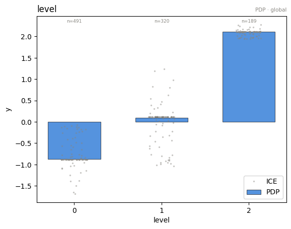
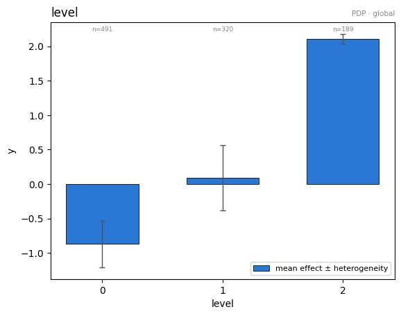
PDP: bars at the levels, ICE as jittered dots
For a discrete feature the model is evaluated only at the observed levels — never at fake in-between values. Verbs take the feature by index or by name — pdp.plot(0) and pdp.plot("level") are the same call; we use the name below.
pdp = effector.PDP(data, model.predict, schema=schema)
pdp.plot("level", heterogeneity="ice", centering=True)
pdp.plot("level", heterogeneity="std", centering=True)
eval follows the same rule — asking for a non-level value is an error:
print(pdp.eval("level", np.array([0.0, 1.0, 2.0]), centering="zero_start"))
try:
    pdp.eval("level", np.array([0.5]))
except ValueError as e:
    print("ValueError:", e)
[0.         0.96102959 2.9805148 ]
ValueError: level is categorical and can only be evaluated at its observed levels [0.0, 1.0, 2.0]; got invalid value(s) [0.5]
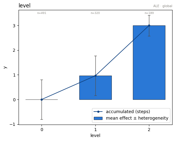
ALE: adjacent-level differences, accumulated
Each bar is the accumulated effect at a level; the whisker is the standard deviation of the step into that level. For an ordinal feature this is exact — the model is only queried at real levels.
ale = effector.ALE(data, model.predict, schema=schema)
ale.plot("level", centering="zero_start")
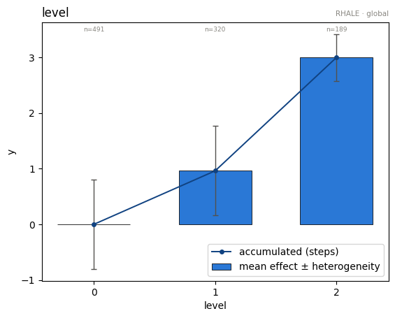
RHALE: adaptive level grouping
On ordinal features RHALE treats the adjacent-level differences as a discrete derivative and lets Greedy/DP binning merge neighboring transitions with similar effect — useful for high-cardinality ordinal features.
rhale = effector.RHALE(data, model.predict, model.jacobian, schema=schema)
rhale.fit(0, binning_method="greedy", centering="zero_start")
rhale.plot("level", centering="zero_start")
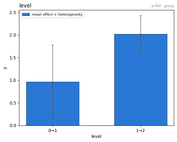
DerPDP differentiates discretely
On a discrete axis the derivative becomes the finite difference: for every instance, the change in prediction when the level switches to the next one. The jacobian is never used there — the bars below are per-transition means (± std) of the plain ICE differences, labeled v→w.
derpdp = effector.DerPDP(data, model.predict, model.jacobian, schema=schema)
derpdp.plot("level", heterogeneity="std")
print("heter_score:", round(derpdp.heter_score(0), 3))
print("importance :", round(derpdp.importance(0), 3))
heter_score: 0.58
importance : 0.891
Importance and one-click explanation
Every global effect exposes importances() — the per-feature dispersion of the mean effect (the μ-twin of heterogeneity), a scalar summary of how much each feature moves the prediction. effector.explain(...) wraps the whole tour into a serializable Report with a self-contained HTML view.
# per-feature importance = dispersion of the mean effect (the mu-twin of heterogeneity)
print("importances:", np.round(pdp.importances(), 3))

# one-click auto-explanation -> Report (serializable; self-contained HTML)
report = effector.explain(data, model.predict, method="pdp", schema=schema, nof_instances="all")
report.show()

# the whole notebook, in one page: the report published with this example
from pathlib import Path
_out = Path("reports") / "08_categorical_features"
_out.mkdir(parents=True, exist_ok=True)
report.to_html(_out / "report_pdp.html")
importances: [1.103 0.039 0.007]
[effector] global effects   (GAM)  -> 90.5% of the model's variance
           regional effects (CALM) -> 98.4%

  ════════════════════════════════════════════════════════════════════════
  PDP report  ·  target: y
  ════════════════════════════════════════════════════════════════════════

  DATA & MODEL
  ────────────────────────────────────────────────────────────────────────
    instances     1,000
    features      3  ·  1 ordinal · 2 continuous
    model output  mean 0.875 · std 1.17 · range [-0.993, 3]

  EXPLAINED VARIANCE
  ────────────────────────────────────────────────────────────────────────
    step         split on                 solo     ΔR²      R²       heter
    ──────────────────────────────────────────────────────────────────────
    GAM          (all features global)       —       —   90.5%           —
  + x1           level, x2               +7.9%   +7.9%   98.4% 0.37 → 0.08
    ──────────────────────────────────────────────────────────────────────
    FINAL                                                98.4%

  REJECTED SPLITS                                            min gain 1.0%
  ────────────────────────────────────────────────────────────────────────
    feature      split on                 solo     ΔR²    reason
    ──────────────────────────────────────────────────────────────────────
  ✗ level        x1, x2                  +7.0%   -4.8%    redundant

    ✗ redundant: it would explain variance on its own (see solo),
      but the accepted splits already account for it.

  FEATURES                                ranked, in the selected snapshot
  ────────────────────────────────────────────────────────────────────────
    feature        importance                          heter      #regions
    ──────────────────────────────────────────────────────────────────────
    level              1.1028  ██████████████████     0.3607             1
    x1                 0.2291  ████                   0.0757             3
    ──────────────────────────────────────────────────────────────────────
    the features above carry 99% of the total importance mass


Feature 1 - Full partition tree:
🌳 Full Tree Structure:
───────────────────────
x1 🔹 [id: 0 | heter: 0.37 | inst: 1000 | w: 1.00]
    x2 < 0.00 🔹 [id: 1 | heter: 0.00 | inst: 498 | w: 0.50]
    x2 ≥ 0.00 🔹 [id: 2 | heter: 0.51 | inst: 502 | w: 0.50]
        level = 0.00 🔹 [id: 3 | heter: 0.00 | inst: 233 | w: 0.23]
        level ∈ {1.00, 2.00} 🔹 [id: 4 | heter: 0.28 | inst: 269 | w: 0.27]
--------------------------------------------------
Feature 1 - Statistics per tree level:
🌳 Tree Summary:
─────────────────
Level 0🔹heter: 0.37
    Level 1🔹heter: 0.26 | 🔻0.11 (31.02%)
        Level 2🔹heter: 0.08 | 🔻0.18 (70.34%)


/home/givasile/github/packages/effector/effector/report.py:606: UserWarning: This figure includes Axes that are not compatible with tight_layout, so results might be incorrect.
  fig.tight_layout()
Regional effects on a categorical feature
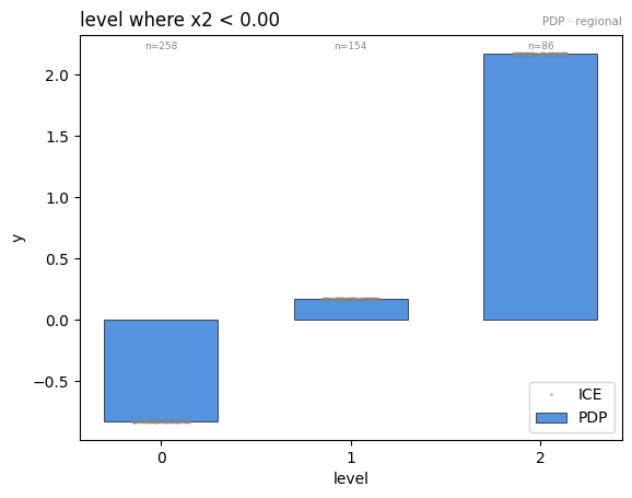
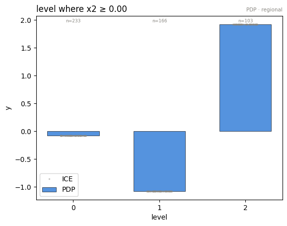
For which subgroups is the per-level effect stable? We use \(f(x) = a_{x_0} + b_{x_0}\,\mathbb{1}_{x_2>0}\): the level effect is unstable globally, but perfectly stable once you condition on the \(x_2\) gate.
A, B = models.ConditionalCategorical.A, models.ConditionalCategorical.B

def gated_model(x):
    codes = x[:, 0].astype(int)
    return A[codes] + B[codes] * (x[:, 2] > 0)

pdp_reg = effector.PDP(data, gated_model, schema=schema, nof_instances="all")
pdp_reg.fit(0, centering=True)
finder = effector.space_partitioning.Best(max_depth=1)
partitions = {0: pdp_reg.find_regions(0, finder=finder)}
partitions[0].show()
Feature 0 - Full partition tree:
🌳 Full Tree Structure:
───────────────────────
level 🔹 [id: 0 | heter: 0.44 | inst: 1000 | w: 1.00]
    x2 < 0.00 🔹 [id: 1 | heter: 0.00 | inst: 498 | w: 0.50]
    x2 ≥ 0.00 🔹 [id: 2 | heter: 0.00 | inst: 502 | w: 0.50]
--------------------------------------------------
Feature 0 - Statistics per tree level:
🌳 Tree Summary:
─────────────────
Level 0🔹heter: 0.44
    Level 1🔹heter: 0.00 | 🔻0.44 (100.00%)
partitions[0].plot(1, heterogeneity="ice", centering=True)
partitions[0].plot(2, heterogeneity="ice", centering=True)
Nominal features from a pandas DataFrame
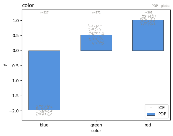
effector is numpy-only, so a DataFrame is converted at the door with effector.from_dataframe(df), which returns (X, schema): X is the encoded (N, D) numpy matrix and schema carries the feature types and the category labels. Your model stays a plain numpy→numpy callable (it receives the encoded codes). Plots translate the codes back to the category labels via the schema.
N2 = 800
color = rng.choice(["red", "green", "blue"], N2, p=[0.4, 0.35, 0.25])
df = pd.DataFrame({
    "color": pd.Categorical(color),
    "x1": rng.uniform(-1, 1, N2),
})

# effector is numpy-only: convert the DataFrame to (X, schema) at the door.
X, schema_nominal = effector.from_dataframe(df)
levels = list(schema_nominal.category_names[0].values())  # the names by code: ['blue', 'green', 'red']

# the model is numpy->numpy; it receives the encoded codes in column 0.
color_effect = {"red": 2.0, "green": 1.5, "blue": -1.0}
effect_by_code = np.array([color_effect[name] for name in levels])
green_code = levels.index("green")

def np_model(x):
    codes = x[:, 0].astype(int)
    return effect_by_code[codes] + 0.5 * x[:, 1] * (codes == green_code)

pdp_nominal = effector.PDP(X, np_model, schema=schema_nominal)
pdp_nominal.plot(0, heterogeneity="ice", centering=True)
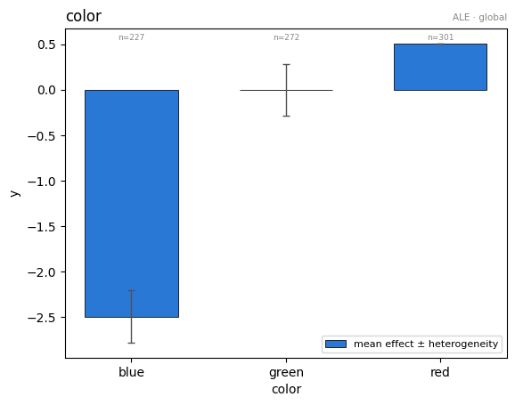
ALE on a nominal feature: the order caveat
ALE accumulates along an order that nominal features do not have. By default effector uses the ascending encoded order and the curve's shape depends on it — the meaningful quantities are the adjacent-level differences. You can declare the order (order=[...]) or induce it from the other features (order="similarity", Kolmogorov–Smirnov seriation):
ale_nominal = effector.ALE(X, np_model, schema=schema_nominal)
ale_nominal.fit(0, centering="zero_start", order="similarity")
ale_nominal.plot(0, centering="zero_start")
Takeaways
- Declare
feature_typesin theschemawhenever you know them — inference is a fallback, not an oracle. - PDP/ShapDP treat ordinal and nominal identically (order-free math); ALE needs an order; RHALE groups adjacent levels only when the order is real (ordinal) and falls back to plain ALE on nominal.
- DerPDP differentiates discretely: per-transition ICE differences, never the jacobian.
heter_score/importanceare std-type scalars in output units (the units contract) — comparable across feature types and, in magnitude, across methods; for nominal features they are order-free (all level pairs).- Regional effects answer stability questions per level — heterogeneity is frequency-weighted over the levels.
- The exact formulas per method and feature type live in
docs/guides/method_semantics.md.
Cross-method sanity check
The one-liner effector.explain with every engine this notebook's model
supports. Everything must run end to end; the closing table puts the reads
side by side. Where methods disagree — ranking, accepted splits, R² — that is
a property of the data/model worth a closer look, not an error.
from pathlib import Path
_out = Path("reports") / "08_categorical_features"
_out.mkdir(parents=True, exist_ok=True)

# === cross-method sweep: effector.explain on every applicable engine ======
sweep_reports = {}
for _m in ["pdp", "derpdp", "ale", "rhale", "shapdp"]:
    _kw = {"nof_instances": 300} if _m == "shapdp" else {}
    print(f"--- {_m} " + "-" * 50)
    sweep_reports[_m] = effector.explain(
        data, model.predict, model.jacobian, method=_m, schema=schema, **_kw
    )
    if _m != "pdp":  # the published report is the narrated one above
        sweep_reports[_m].to_html(_out / f"report_{_m}.html")

print()
print(f"{'method':<8} {'ranking (plotted)':<44} {'GAM R2':>8} {'final R2':>9}  splits")
for _m, _r in sweep_reports.items():
    _rank = " > ".join(fr.name for fr in _r.features)
    _ev = _r.explained_variance
    if _ev:
        _sp = "; ".join(f"{s['name']} on {s['on']}" for s in _ev["stages"]) or "none"
        print(f"{_m:<8} {_rank:<44} {_ev['gam_r2']:>7.1%} {_ev['regional_r2']:>8.1%}  {_sp}")
    else:
        print(f"{_m:<8} {_rank:<44} {'-':>7} {'-':>8}  (derivative scale: no variance ledger)")

print(f"\nreports stored in {_out}/")
--- pdp --------------------------------------------------
[effector] global effects   (GAM)  -> 90.5% of the model's variance
           regional effects (CALM) -> 98.4%
--- derpdp --------------------------------------------------


/home/givasile/github/packages/effector/effector/report.py:606: UserWarning: This figure includes Axes that are not compatible with tight_layout, so results might be incorrect.
  fig.tight_layout()


--- ale --------------------------------------------------
[effector] global effects   (GAM)  -> 90.3% of the model's variance
           regional effects (CALM) -> 97.4%


/home/givasile/github/packages/effector/effector/report.py:606: UserWarning: This figure includes Axes that are not compatible with tight_layout, so results might be incorrect.
  fig.tight_layout()


--- rhale --------------------------------------------------
[effector] global effects   (GAM)  -> 90.5% of the model's variance
           regional effects (CALM) -> 98.4%


/home/givasile/github/packages/effector/effector/report.py:606: UserWarning: This figure includes Axes that are not compatible with tight_layout, so results might be incorrect.
  fig.tight_layout()


--- shapdp --------------------------------------------------


[effector] global effects   (GAM)  -> 90.4% of the model's variance
           regional effects (CALM) -> 98.2%


/home/givasile/github/packages/effector/effector/report.py:606: UserWarning: This figure includes Axes that are not compatible with tight_layout, so results might be incorrect.
  fig.tight_layout()


method   ranking (plotted)                              GAM R2  final R2  splits
pdp      level > x1                                     90.5%    98.4%  x1 on level, x2
derpdp   level                                              -        -  (derivative scale: no variance ledger)
ale      level                                          90.3%    97.4%  level on x1, x2
rhale    level > x1                                     90.5%    98.4%  x1 on level, x2
shapdp   level > x1                                     90.4%    98.2%  x1 on level, x2; level on x1, x2

reports stored in reports/08_categorical_features/