One-click explanations: importance, explain, and the Report
- Author: givasile
- Runtime: ~10 s
- Description: A tour of the new high-level API on a known synthetic model:
per-feature importance, the one-click
effector.explain(...)orchestrator, the serializableReportvalue object (show/plot_importance/to_html), and drilling into a heterogeneous feature withfind_regions→Partition. - 📄 The whole notebook in one page: PDP report
In the earlier tutorials we constructed each effect method by hand, fitted it, and read the
plots one feature at a time. effector now offers a high-level layer that automates the whole
triage: rank features by importance → plot the important ones → automatically split the
heterogeneous ones into regions, all returned as a single serializable Report.
import numpy as np
import effector
A known black-box model
We use a gated interaction on \(D=3\) features, \(x_0,x_1\sim\mathcal{U}(-1,1)\) and \(x_2\in\{0,1\}\):
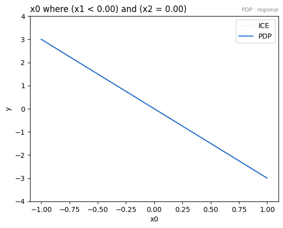
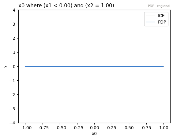
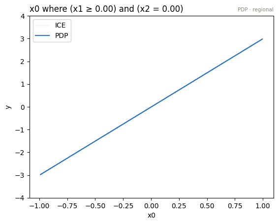
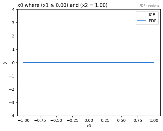
- \(x_0\) has a strong but heterogeneous effect: its slope flips with \(\operatorname{sign}(x_1)\) and switches off when \(x_2=1\). Globally its mean effect nearly cancels, but it splits cleanly into regions.
- \(x_1\) has a weak, homogeneous effect (\(0.4x_1\)).
- \(x_2\) only gates — no direct additive effect.
This is exactly the situation the report is meant to triage.
rng = np.random.default_rng(0)
N = 3000
x0 = rng.uniform(-1, 1, N)
x1 = rng.uniform(-1, 1, N)
x2 = rng.integers(0, 2, N).astype(float)
X = np.stack([x0, x1, x2], axis=1)

def model(X):
    gate = np.where(X[:, 2] == 0, 1.0, 0.0)
    return gate * np.where(X[:, 1] > 0, 1.0, -1.0) * X[:, 0] * 3.0 + 0.4 * X[:, 1]

def model_jac(X):
    g = np.zeros_like(X)
    gate = np.where(X[:, 2] == 0, 1.0, 0.0)
    g[:, 0] = gate * np.where(X[:, 1] > 0, 1.0, -1.0) * 3.0
    g[:, 1] = 0.4
    return g

# x2 is a binary gate -> declare it nominal so derivative/binning methods treat it as a category
schema = {"feature_names": ["x0", "x1", "x2"],
          "feature_types": ["continuous", "continuous", "nominal"],
          "target_name": "y"}
1. Feature importance
importance(feature, mask=None) is the dispersion of the mean effect of a feature — the
\(\mu\)-twin of heter_score (which measures the spread of the per-instance effect). It is
model-free (re-summarised from the cached local effects), centering-invariant, and data-weighted.
importances() returns the whole per-feature vector.
pdp = effector.PDP(X, model, schema=schema, nof_instances="all")
pdp.fit("all")

for f, name in enumerate(schema["feature_names"]):
    print(f"{name}:  importance={pdp.importance(f):.3f}   heter_score={pdp.heter_score(f):.3f}")

print("\nimportances() vector:", np.round(pdp.importances(), 3))
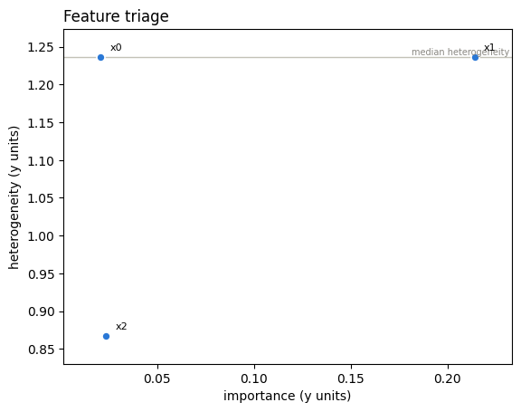
x0:  importance=0.021   heter_score=1.236
x1:  importance=0.214   heter_score=1.237
x2:  importance=0.024   heter_score=0.867

importances() vector: [0.021 0.214 0.024]
Importance and heterogeneity are orthogonal axes. Note that \(x_0\) scores low importance
but high heter_score: because its slope flips with \(\operatorname{sign}(x_1)\), the mean
effect nearly cancels over the data (low dispersion of the mean = low importance), yet the
per-instance effects are wildly spread (high heterogeneity). This is precisely the feature a
global average hides and a regional analysis reveals. \(x_1\) carries a genuine mean effect;
\(x_2\) only gates. explain uses both axes: it plots the features with the largest mean effect and
automatically runs find_regions on the ones whose heterogeneity is high.
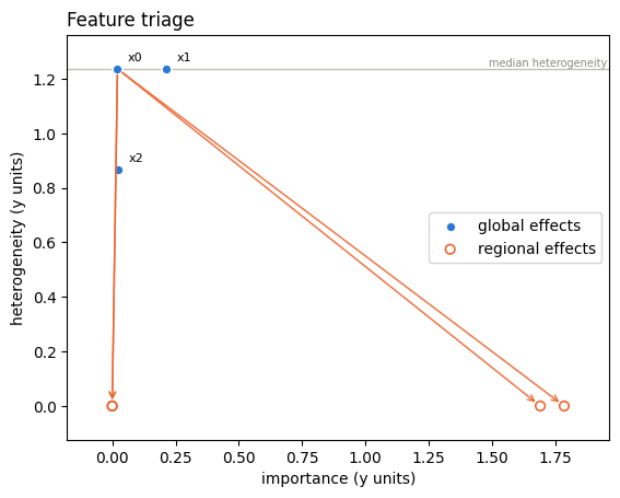
effector.plot_triage draws this survey as one picture — the manual counterpart of what explain automates. Importance right, heterogeneity up: the top-right corner is where the mean effect hides something.
effector.plot_triage(pdp)
2. effector.explain(...) → Report
explain runs the entire pipeline in one model-touch: fit → rank by importance → build the
top-\(k\) curves → find_regions on the features whose heterogeneity exceeds a threshold. It
returns a Report — a serializable value (it owns the computed arrays, not a live reference
to the estimator).
report = effector.explain(X, model, method="pdp", schema=schema,
                          top_k=3, nof_instances="all")
report.show()
[effector] global effects   (GAM)  -> 2.7% of the model's variance
           regional effects (CALM) -> 100.0%

  ════════════════════════════════════════════════════════════════════════
  PDP report  ·  target: y
  ════════════════════════════════════════════════════════════════════════

  DATA & MODEL
  ────────────────────────────────────────────────────────────────────────
    instances     3,000
    features      3  ·  2 continuous · 1 nominal
    model output  mean 0.0223 · std 1.25 · range [-3.31, 3.29]

  EXPLAINED VARIANCE
  ────────────────────────────────────────────────────────────────────────
    step         split on                 solo     ΔR²      R²       heter
    ──────────────────────────────────────────────────────────────────────
    GAM          (all features global)       —       —    2.7%           —
  + x0           x1, x2                 +97.3%  +97.3%  100.0% 1.24 → 0.00
    ──────────────────────────────────────────────────────────────────────
    FINAL                                               100.0%

  REJECTED SPLITS                                            min gain 1.0%
  ────────────────────────────────────────────────────────────────────────
    feature      split on                 solo     ΔR²    reason
    ──────────────────────────────────────────────────────────────────────
  ✗ x1           x0, x2                 +71.9%  -71.0%    redundant

    ✗ redundant: it would explain variance on its own (see solo),
      but the accepted splits already account for it.

  FEATURES                                ranked, in the selected snapshot
  ────────────────────────────────────────────────────────────────────────
    feature        importance                          heter      #regions
    ──────────────────────────────────────────────────────────────────────
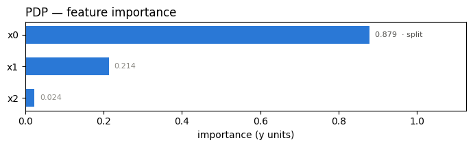
    x0                 0.8794  ██████████████████     0.0000             4
    x1                 0.2141  ████                   1.2365             1
    ──────────────────────────────────────────────────────────────────────
    the features above carry 98% of the total importance mass


Feature 0 - Full partition tree:
🌳 Full Tree Structure:
───────────────────────
x0 🔹 [id: 0 | heter: 1.24 | inst: 3000 | w: 1.00]
    x1 < 0.00 🔹 [id: 1 | heter: 0.89 | inst: 1480 | w: 0.49]
        x2 = 0.00 🔹 [id: 2 | heter: 0.00 | inst: 742 | w: 0.25]
        x2 = 1.00 🔹 [id: 3 | heter: 0.00 | inst: 738 | w: 0.25]
    x1 ≥ 0.00 🔹 [id: 4 | heter: 0.85 | inst: 1520 | w: 0.51]
        x2 = 0.00 🔹 [id: 5 | heter: 0.00 | inst: 778 | w: 0.26]
        x2 = 1.00 🔹 [id: 6 | heter: 0.00 | inst: 742 | w: 0.25]
--------------------------------------------------
Feature 0 - Statistics per tree level:
🌳 Tree Summary:
─────────────────
Level 0🔹heter: 1.24
    Level 1🔹heter: 0.87 | 🔻0.37 (29.77%)
        Level 2🔹heter: 0.00 | 🔻0.87 (100.00%)
# horizontal importance bar chart (returns (fig, ax) when show_plot=False)
report.plot_importance()
Self-contained HTML report
to_html renders the whole thing to a single self-contained page — every figure is inlined
as a base64 PNG, so there are no external assets. This is the artefact you would share with a
stakeholder. With a path it writes the file and returns None (so your shell isn't flooded
with a megabyte of markup); call it with no arguments to get the HTML string instead.
from pathlib import Path
_out = Path("reports") / "09_explain_importance_report"
_out.mkdir(parents=True, exist_ok=True)

report.to_html(_out / "report_pdp.html")        # writes the file, returns None
html = open(_out / "report_pdp.html").read()  # the raw markup, if you want to poke at it
print("inlined figures:", "data:image/png;base64" in html)
print("no external assets:", "http://" not in html and "https://" not in html)
print("length (chars):", len(html))
/home/givasile/github/packages/effector/effector/report.py:606: UserWarning: This figure includes Axes that are not compatible with tight_layout, so results might be incorrect.
  fig.tight_layout()


inlined figures: True
no external assets: True
length (chars): 478167
The Report is a value: it round-trips without the model
to_dict / from_dict serialise the report; a reloaded report can still render its text and the
importance chart (the live-plot sugar that needs the estimator raises a clear error when unbound).
from effector import Report

reloaded = Report.from_dict(report.to_dict())
print("feature order preserved:", [fr.name for fr in reloaded.features])
reloaded.show()
feature order preserved: ['x0', 'x1']

  ════════════════════════════════════════════════════════════════════════
  PDP report  ·  target: y
  ════════════════════════════════════════════════════════════════════════

  DATA & MODEL
  ────────────────────────────────────────────────────────────────────────
    instances     3,000
    features      3  ·  2 continuous · 1 nominal
    model output  mean 0.0223 · std 1.25 · range [-3.31, 3.29]

  EXPLAINED VARIANCE
  ────────────────────────────────────────────────────────────────────────
    step         split on                 solo     ΔR²      R²       heter
    ──────────────────────────────────────────────────────────────────────
    GAM          (all features global)       —       —    2.7%           —
  + x0           x1, x2                 +97.3%  +97.3%  100.0% 1.24 → 0.00
    ──────────────────────────────────────────────────────────────────────
    FINAL                                               100.0%

  REJECTED SPLITS                                            min gain 1.0%
  ────────────────────────────────────────────────────────────────────────
    feature      split on                 solo     ΔR²    reason
    ──────────────────────────────────────────────────────────────────────
  ✗ x1           x0, x2                 +71.9%  -71.0%    redundant

    ✗ redundant: it would explain variance on its own (see solo),
      but the accepted splits already account for it.

  FEATURES                                ranked, in the selected snapshot
  ────────────────────────────────────────────────────────────────────────
    feature        importance                          heter      #regions
    ──────────────────────────────────────────────────────────────────────
    x0                 0.8794  ██████████████████     0.0000             4
    x1                 0.2141  ████                   1.2365             1
    ──────────────────────────────────────────────────────────────────────
    the features above carry 98% of the total importance mass


Feature 0 - Full partition tree:
🌳 Full Tree Structure:
───────────────────────
x0 🔹 [id: 0 | heter: 1.24 | inst: 3000 | w: 1.00]
    x1 < 0.00 🔹 [id: 1 | heter: 0.89 | inst: 1480 | w: 0.49]
        x2 = 0.00 🔹 [id: 2 | heter: 0.00 | inst: 742 | w: 0.25]
        x2 = 1.00 🔹 [id: 3 | heter: 0.00 | inst: 738 | w: 0.25]
    x1 ≥ 0.00 🔹 [id: 4 | heter: 0.85 | inst: 1520 | w: 0.51]
        x2 = 0.00 🔹 [id: 5 | heter: 0.00 | inst: 778 | w: 0.26]
        x2 = 1.00 🔹 [id: 6 | heter: 0.00 | inst: 742 | w: 0.25]
--------------------------------------------------
Feature 0 - Statistics per tree level:
🌳 Tree Summary:
─────────────────
Level 0🔹heter: 1.24
    Level 1🔹heter: 0.87 | 🔻0.37 (29.77%)
        Level 2🔹heter: 0.00 | 🔻0.87 (100.00%)
3. Drilling into a heterogeneous feature: find_regions → Partition
The report already ran find_regions on the heterogeneous features. We can also call it directly:
it returns a Partition (a value object) and stores nothing on the effect. The heterogeneity a
Partition reports is heter_score(feature, mask) on each region's mask.
part = pdp.find_regions(0, finder="best")
part.show()
Feature 0 - Full partition tree:
🌳 Full Tree Structure:
───────────────────────
x0 🔹 [id: 0 | heter: 1.24 | inst: 3000 | w: 1.00]
    x1 < 0.00 🔹 [id: 1 | heter: 0.89 | inst: 1480 | w: 0.49]
        x2 = 0.00 🔹 [id: 2 | heter: 0.00 | inst: 742 | w: 0.25]
        x2 = 1.00 🔹 [id: 3 | heter: 0.00 | inst: 738 | w: 0.25]
    x1 ≥ 0.00 🔹 [id: 4 | heter: 0.85 | inst: 1520 | w: 0.51]
        x2 = 0.00 🔹 [id: 5 | heter: 0.00 | inst: 778 | w: 0.26]
        x2 = 1.00 🔹 [id: 6 | heter: 0.00 | inst: 742 | w: 0.25]
--------------------------------------------------
Feature 0 - Statistics per tree level:
🌳 Tree Summary:
─────────────────
Level 0🔹heter: 1.24
    Level 1🔹heter: 0.87 | 🔻0.37 (29.77%)
        Level 2🔹heter: 0.00 | 🔻0.87 (100.00%)
# a Partition supports len / iteration / indexing; regions carry mask, heterogeneity, weight, ...
print("number of regions:", len(part))
print("leaves:", [r.idx for r in part.leaves])
for r in part:
    print(f"  region {r.idx}: level={r.level}  inst={r.nof_instances}  heter={r.heterogeneity:.3f}")
number of regions: 7
leaves: [2, 3, 5, 6]
  region 0: level=0  inst=3000  heter=1.236
  region 1: level=1  inst=1480  heter=0.888
  region 2: level=2  inst=742  heter=0.000
  region 3: level=2  inst=738  heter=0.000
  region 4: level=1  inst=1520  heter=0.849
  region 5: level=2  inst=778  heter=0.000
  region 6: level=2  inst=742  heter=0.000
# plot each leaf region: the gated interaction resolves into clean, homogeneous lines
for r in part.leaves:
    part.plot(r.idx, heterogeneity="ice", centering=True, y_limits=[-4, 4])
And the before/after in one figure: arrows from the global point to the leaves — right and down, importance up, heterogeneity explained.
effector.plot_triage(pdp, partitions={"x0": part})
4. Same pipeline, any method
explain accepts method="pdp" | "ale" | "rhale" | "shapdp" (and "derpdp"); pass
model_jac= for the derivative-based methods. The importance ranking is method-agnostic — the
important feature stays on top.
for method in ["pdp", "ale", "rhale", "shapdp"]:
    kw = {"schema": schema, "top_k": 3, "nof_instances": "all"}
    if method in ("rhale",):
        kw["model_jac"] = model_jac
    if method == "shapdp":
        kw["nof_instances"] = 500  # keep SHAP cheap
    rep = effector.explain(X, model, method=method, **kw)
    ranked = [(fr.name, round(fr.importance, 3)) for fr in rep.features]
    print(f"{method:7s} -> {ranked}")
[effector] global effects   (GAM)  -> 2.7% of the model's variance
           regional effects (CALM) -> 100.0%
pdp     -> [('x0', 0.879), ('x1', 0.214)]
[effector] global effects   (GAM)  -> 2.5% of the model's variance
           regional effects (CALM) -> 100.0%
ale     -> [('x0', 0.879), ('x1', 0.228)]
[effector] global effects   (GAM)  -> 2.7% of the model's variance
           regional effects (CALM) -> 100.0%
rhale   -> [('x0', 0.879), ('x1', 0.231)]


[effector] global effects   (GAM)  -> 0.1% of the model's variance
           regional effects (CALM) -> 87.1%
shapdp  -> [('x0', 0.435), ('x1', 0.408)]
Takeaways
importance(feature)/importances()give a method-agnostic ranking of feature effect strength.effector.explain(...)triages a model in one call and returns a serializableReport.Report.to_html(path)produces a single self-contained page to share.find_regions(feature) -> Partitionis the queryable, value-based regional API:show,plot,eval,leaves,to_dict— nothing is stored on the estimator.
Cross-method sanity check
The one-liner effector.explain with every engine this notebook's model
supports. Everything must run end to end; the closing table puts the reads
side by side. Where methods disagree — ranking, accepted splits, R² — that is
a property of the data/model worth a closer look, not an error.
from pathlib import Path
_out = Path("reports") / "09_explain_importance_report"
_out.mkdir(parents=True, exist_ok=True)

# === cross-method sweep: effector.explain on every applicable engine ======
sweep_reports = {}
for _m in ["pdp", "derpdp", "ale", "rhale", "shapdp"]:
    _kw = {"nof_instances": 300} if _m == "shapdp" else {}
    print(f"--- {_m} " + "-" * 50)
    sweep_reports[_m] = effector.explain(
        X, model, model_jac, method=_m, schema=schema, **_kw
    )
    if _m != "pdp":  # the published report is the narrated one above
        sweep_reports[_m].to_html(_out / f"report_{_m}.html")

print()
print(f"{'method':<8} {'ranking (plotted)':<44} {'GAM R2':>8} {'final R2':>9}  splits")
for _m, _r in sweep_reports.items():
    _rank = " > ".join(fr.name for fr in _r.features)
    _ev = _r.explained_variance
    if _ev:
        _sp = "; ".join(f"{s['name']} on {s['on']}" for s in _ev["stages"]) or "none"
        print(f"{_m:<8} {_rank:<44} {_ev['gam_r2']:>7.1%} {_ev['regional_r2']:>8.1%}  {_sp}")
    else:
        print(f"{_m:<8} {_rank:<44} {'-':>7} {'-':>8}  (derivative scale: no variance ledger)")

print(f"\nreports stored in {_out}/")
--- pdp --------------------------------------------------
[effector] global effects   (GAM)  -> 2.7% of the model's variance
           regional effects (CALM) -> 100.0%
--- derpdp --------------------------------------------------


/home/givasile/github/packages/effector/effector/report.py:606: UserWarning: This figure includes Axes that are not compatible with tight_layout, so results might be incorrect.
  fig.tight_layout()


--- ale --------------------------------------------------
[effector] global effects   (GAM)  -> 2.5% of the model's variance
           regional effects (CALM) -> 100.0%


/home/givasile/github/packages/effector/effector/report.py:606: UserWarning: This figure includes Axes that are not compatible with tight_layout, so results might be incorrect.
  fig.tight_layout()


--- rhale --------------------------------------------------
[effector] global effects   (GAM)  -> 2.7% of the model's variance
           regional effects (CALM) -> 100.0%


/home/givasile/github/packages/effector/effector/report.py:606: UserWarning: This figure includes Axes that are not compatible with tight_layout, so results might be incorrect.
  fig.tight_layout()


--- shapdp --------------------------------------------------


[effector] global effects   (GAM)  -> -0.6% of the model's variance
           regional effects (CALM) -> 87.3%


/home/givasile/github/packages/effector/effector/report.py:606: UserWarning: This figure includes Axes that are not compatible with tight_layout, so results might be incorrect.
  fig.tight_layout()


method   ranking (plotted)                              GAM R2  final R2  splits
pdp      x0 > x1                                         2.7%   100.0%  x0 on x1, x2
derpdp   x1                                                 -        -  (derivative scale: no variance ledger)
ale      x0 > x1                                         2.5%   100.0%  x0 on x1, x2
rhale    x0 > x1                                         2.7%   100.0%  x0 on x1, x2
shapdp   x0 > x1                                        -0.6%    87.3%  x0 on x1, x2; x1 on x0, x2

reports stored in reports/09_explain_importance_report/