Customize .fit()

Effector is designed to work well with its default settings, but it also allows for customization if the user needs more control over the processing steps. This flexibility is achieved through the use of the .fit() routine, which offers a range of options for customizing each global or regional effect method

Dataset

Create a dataset with 3 features, uniformly distributed in the range [-1, 1].

dist = effector.datasets.IndependentUniform(dim=3, low=-1, high=1)
X_test = dist.generate_data(n=200)
axis_limits = dist.axis_limits

Black-box model and Jacobian

Construct a black-box model with a double conditional interaction: \(x_1\) effect interacts with \(x_2\) and \(x_3\).

\[ f(x_1, x_2, x_3) = -3x_1^2\mathbb{1}_{x_2 < 0}\mathbb{1}_{x_3 < 0} \ +x_1^2\mathbb{1}_{x_2 < 0}\mathbb{1}_{x_3 \geq 0} \ -e^{x_1}\mathbb{1}_{x_2 \geq 0}\mathbb{1}_{x_3 < 0} \ +e^{3x_1}\mathbb{1}_{x_2 \geq 0}\mathbb{1}_{x_3 \geq 0} \]

model = effector.models.DoubleConditionalInteraction()
predict = model.predict
jacobian = model.jacobian

Global Effect

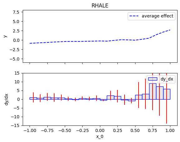
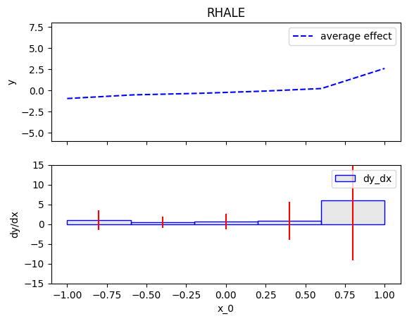
We will compute the global effect of the first feature using the RHALE method. First, we will use the default settings of the .fit() routine, which automatically partitions the feature space into bins. Then, we will customize the .fit() routine to use a number of 5 equal-width bins.

RHALE

Default settingsCustomized .fit()

rhale = effector.RHALE(X_test, predict, jacobian, axis_limits=axis_limits, nof_instances="all")
rhale.plot(feature=0, y_limits=y_limits, dy_limits=dy_limits)

rhale = effector.RHALE(X_test, predict, jacobian, axis_limits=axis_limits, nof_instances="all")
rhale.fit(features=0, binning_method=effector.axis_partitioning.Fixed(nof_bins=5))
rhale.plot(feature=0, y_limits=y_limits, dy_limits=dy_limits)

Regional Effect

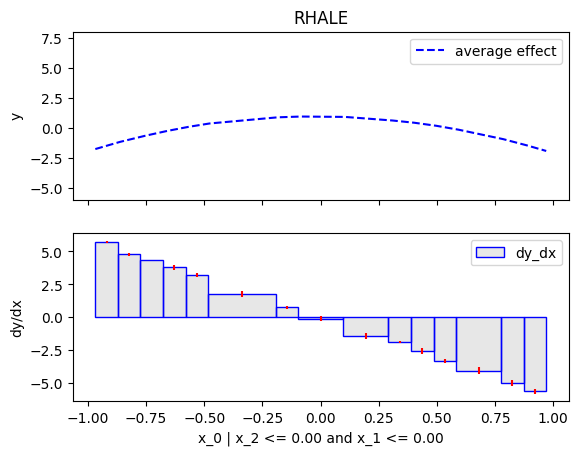
Similarly, we will compute the regional effect of the first feature using the RHALE method. We will first use the default settings of the .fit() routine, which automatically partitions the feature space into bins and goes until depth=2 of the partition tree. Then, we will customize the .fit() routine to use a number of 5 equal-width bins and go until depth=1 of the partition tree.

RHALE

init()

Default settingsCustomized .fit()

r_rhale = effector.RegionalRHALE(X_test, predict, jacobian, axis_limits=axis_limits, nof_instances="all")
r_rhale.summary(0)

rhale = effector.RHALE(X_test, predict, jacobian, axis_limits=axis_limits, nof_instances="all")
rhale.fit(features=0, binning_method=effector.axis_partitioning.Fixed(nof_bins=5))
rhale.plot(feature=0, y_limits=y_limits, dy_limits=dy_limits)

.summary() output

Default settingsCustomized .fit()

Feature 0 - Full partition tree:
🌳 Full Tree Structure:
───────────────────────
x_0 🔹 [id: 0 | heter: 60.47 | inst: 200 | w: 1.00]
    x_2 ≤ 0.00 🔹 [id: 1 | heter: 2.36 | inst: 105 | w: 0.53]
        x_1 ≤ 0.00 🔹 [id: 2 | heter: 0.06 | inst: 45 | w: 0.23]
        x_1 > 0.00 🔹 [id: 3 | heter: 0.00 | inst: 60 | w: 0.30]
    x_2 > 0.00 🔹 [id: 4 | heter: 70.28 | inst: 95 | w: 0.47]
        x_1 ≤ 0.00 🔹 [id: 5 | heter: 0.00 | inst: 45 | w: 0.23]
        x_1 > 0.00 🔹 [id: 6 | heter: 8.08 | inst: 50 | w: 0.25]

Feature 0 - Full partition tree:
Node id: 0, name: x_0, heter: 53.64 || nof_instances:   200 || weight: 1.00
        Node id: 1, name: x_0 | x_2 <= 0.0, heter: 2.42 || nof_instances:   105 || weight: 0.53
        Node id: 2, name: x_0 | x_2  > 0.0, heter: 61.95 || nof_instances:    95 || weight: 0.47
--------------------------------------------------
Feature 0 - Statistics per tree level:
Level 0, heter: 53.64
        Level 1, heter: 30.70 || heter drop : 22.94 (units), 42.77% (pcg)

.plot()

Default settingsCustomized .fit()

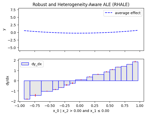
node_idx=3: \(x_0\) when \(x_1 \leq 0\) and \(x_2 \leq 0\)	node_idx=4: \(x_0\) when \(x_1 > 0\) and \(x_2 \leq 0\)
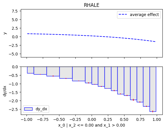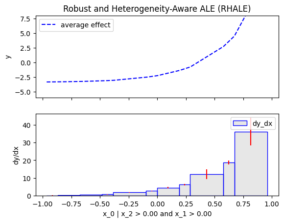
node_idx=5: \(x_0\) when \(x_1 \leq 0\) and \(x_2 > 0\)	node_idx=6: \(x_0\) when \(x_1 > 0\) and \(x_2 > 0\)

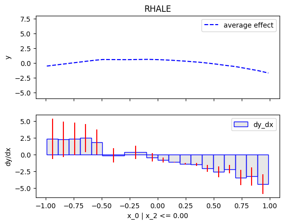
rhale.plot(feature=0, node_idx=1, y_limits=y_limits, dy_limits=dy_limits)
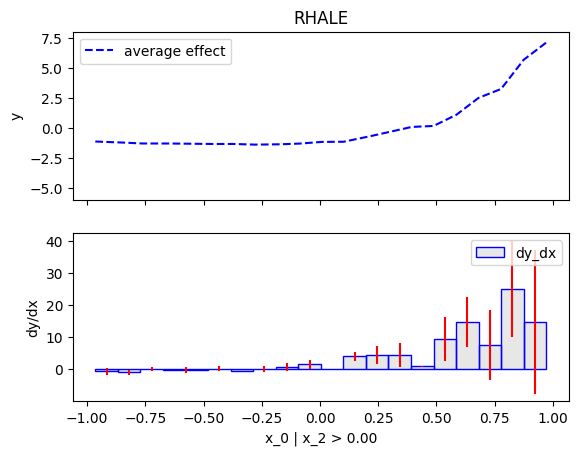
rhale.plot(feature=0, node_idx=2, y_limits=y_limits, dy_limits=dy_limits)

node_idx=1: \(x_0\) when \(x_2 \leq 0\)	node_idx=2: \(x_0\) when \(x_2 > 0\)