Customize .fit()
Description
Part of the interactive API guide:
what the .fit() knobs actually change.
Construct and fit lists them; this page shows
them at work on a model built to punish bad defaults.
Reading time
Approx. 4' to read.
The rig
A synthetic model with a double conditional interaction: the effect of \(x_1\) flips shape with the signs of both \(x_2\) and \(x_3\).
dist = effector.datasets.IndependentUniform(dim=3, low=-1, high=1)
X_test = dist.generate_data(n=200)

model = effector.models.DoubleConditionalInteraction()
predict, jacobian = model.predict, model.jacobian
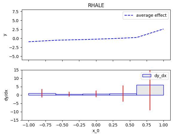
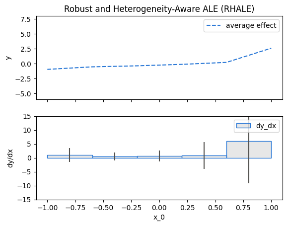
Binning: the global effect's resolution
The accumulation based engines summarize local effects per bin, and the
bins are a fit decision: "dp" (variable size, the RHALE default),
"agglomerative", "quantile", "fixed", or a configured instance from
effector.axis_partitioning.
rhale = effector.RHALE(X_test, predict, jacobian, nof_instances="all")
rhale.plot(feature=0)
rhale = effector.RHALE(X_test, predict, jacobian, nof_instances="all")
rhale.fit(features=0, binning_method=effector.axis_partitioning.Fixed(nof_bins=5))
rhale.plot(feature=0)
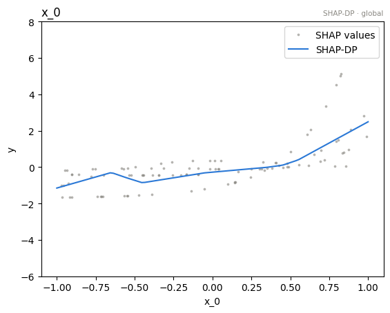
shap_dp = effector.ShapDP(X_test, predict, nof_instances="all")
shap_dp.plot(feature=0)
shap_dp = effector.ShapDP(X_test, predict, nof_instances="all")
shap_dp.fit(features=0, binning_method=effector.axis_partitioning.Fixed(nof_bins=10))
shap_dp.plot(feature=0)
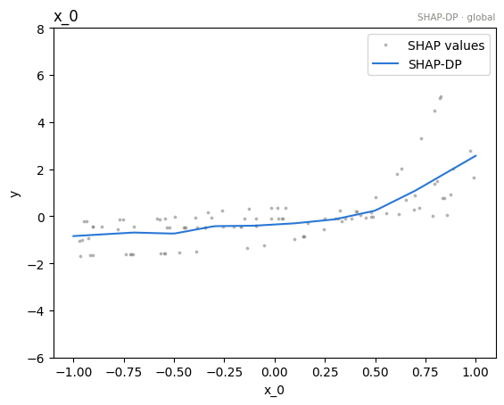
👉 Variable size bins adapt their width to where the effect changes; fixed bins are simpler to reason about and cheaper to eyeball. Binning is pure numpy, so this choice is statistical, not computational; see the efficiency guide.
Fit once, remembered everywhere
The binning declared at fit is replayed by every later query: eval,
plot, heter_score(mask=), the whole region search. That is why the
knobs live on fit and are deliberately not accepted by eval/plot:
one feature, one configuration, no drift.
The finder: the region search's shape
find_regions accepts a configured finder. Best (the default) grows the
tree greedily to max_depth=2; cap it to force a coarser partition:
rhale = effector.RHALE(X_test, predict, jacobian, nof_instances="all")
partition = rhale.find_regions(0)
partition.show()
🌳 Full Tree Structure:
───────────────────────
x_0 🔹 [id: 0 | heter: 4.49 | inst: 200 | w: 1.00]
    x_2 < 0.00 🔹 [id: 1 | heter: 0.90 | inst: 105 | w: 0.53]
        x_1 < 0.00 🔹 [id: 2 | heter: 0.10 | inst: 45 | w: 0.23]
        x_1 ≥ 0.00 🔹 [id: 3 | heter: 0.02 | inst: 60 | w: 0.30]
    x_2 ≥ 0.00 🔹 [id: 4 | heter: 4.44 | inst: 95 | w: 0.47]
        x_1 < 0.00 🔹 [id: 5 | heter: 0.03 | inst: 45 | w: 0.23]
        x_1 ≥ 0.00 🔹 [id: 6 | heter: 1.35 | inst: 50 | w: 0.25]
rhale = effector.RHALE(X_test, predict, jacobian, nof_instances="all")
rhale.fit(features=0, binning_method=effector.axis_partitioning.Fixed(nof_bins=5))
partition = rhale.find_regions(0, finder=effector.space_partitioning.Best(max_depth=1))
partition.show()
🌳 Full Tree Structure:
───────────────────────
x_0 🔹 [id: 0 | heter: 4.31 | inst: 200 | w: 1.00]
    x_2 < 0.00 🔹 [id: 1 | heter: 0.93 | inst: 105 | w: 0.53]
    x_2 ≥ 0.00 🔹 [id: 2 | heter: 4.52 | inst: 95 | w: 0.47]
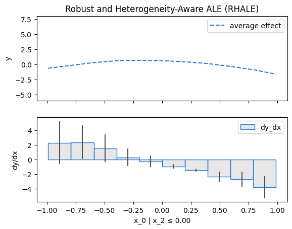
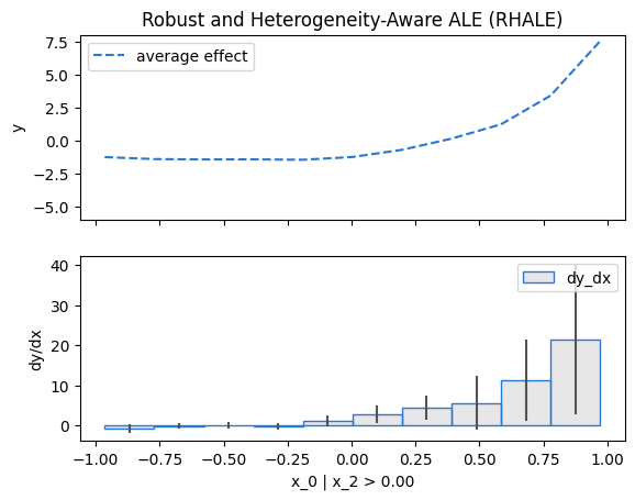
The default search recovers the full 2 level interaction (\(x_2\), then \(x_1\)). The capped search stops at one level, and its two regions are drawable as usual:
partition.plot(1)   # x_0 where x_2 < 0
partition.plot(2)   # x_0 where x_2 ≥ 0
id=1: \(x_0\) where \(x_2 < 0\) |
id=2: \(x_0\) where \(x_2 \geq 0\) |
|---|---|
 |
 |
Beyond max_depth, the finders take numerical_features_grid_size
(candidate split positions per continuous feature) and the search level
strategy is a finder choice: Best (greedy, per node) or BestLevelWise
(one split rule per level). candidate_conditioning_features restricts who
may define splits, on find_regions and select_regions alike.
Where to next
find_regions: the search these knobs steer- Construct and fit: every knob, listed
- The interactive API: back to the guide's map