The interactive API
Description
The in-depth guide to part (c) of effector's API:
construct an engine once, then query it as you go. A map of the verbs;
each verb has its own page.
Reading time
Approx. 5' to read; each verb page is another 4' to 7'.
The lifecycle
flowchart LR
    C["<b>construct</b><br/>PDP(X, model)"] --> F["<b>fit</b><br/><i>the only model touch</i>"]
    F --> Q["<b>query, free</b><br/>plot · eval · importance<br/>heter_score · find_regions"]
    Q -. "zero model calls" .-> F
Construct the engine once; it holds what is expensive. Every question you ask afterwards is answered from cached local effects, without touching the model again.
pdp = effector.PDP(X_test, predict)   # construct
pdp.fit(features="all")               # the only model touch (optional; queries do it lazily)
pdp.plot(0)                           # free
pdp.importance(0)                     # free
pdp.find_regions(0)                   # free
The five engines
They differ in what they compute; they do not differ in how you call them.
pdp    = effector.PDP(X_test, predict)
ale    = effector.ALE(X_test, predict)
rhale  = effector.RHALE(X_test, predict, jacobian)
shapdp = effector.ShapDP(X_test, predict)
derpdp = effector.DerPDP(X_test, predict, jacobian)
The verbs
Every verb has its own in-depth page, on a shared real example (bike sharing, the same run as the report guide) plus a synthetic model where it sharpens the point.
| verb | the question it answers |
|---|---|
PDP(X, model) and .fit() |
which engine, on what data, configured how? |
.plot(f) |
what does feature f do? |
.eval(f, xs) |
…as numbers, on my grid? |
.importance(f) |
how much does f move the output? |
.heter_score(f) |
is the average hiding something? |
.find_regions(f) |
where is it hiding it? |
.select_regions() |
which splits actually earn their keep? |
compare / plot_triage |
do the methods agree, and where to look first? |
The one picture to remember
The running synthetic example is a model with a conditional interaction:
the slope of x_0 flips with the sign of x_1.
pdp = effector.PDP(X_test, predict)
pdp.plot(feature=0)
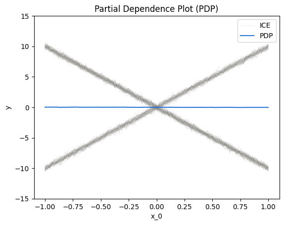
⚠️ The mean curve is flat, and the model is anything but. That flat line
is the average of a +10 slope and a -10 slope cancelling out. The band
around it is screaming; the line is not. That is what heterogeneity is for,
and the whole regional pipeline
(scores →
find_regions →
select_regions) exists to chase it.
It ends where the report begins
parts = pdp.find_regions(features="heterogeneous")
chain = pdp.select_regions(partitions=parts)
This is exactly what the one-liner runs for you; drive it by
hand when you want to hold the values (Partition, CalmSequence) instead
of the frozen Report. The bridge back: pdp.explain() produces the same
Report from your already fitted engine.
Where to next
- The verbs: the seven in-depth pages above
- effector's report: the one-liner, in depth
- The mental model: why the API is shaped this way
- API docs: the reference