plot
Description
Part of the interactive API guide:
effect.plot(feature, ...) on every engine, the heterogeneity views,
centering, and plotting inside a subregion.
Reading time
Approx. 5' to read.
One verb, five engines
The running example is a model with a conditional interaction: the slope
of x_0 flips with the sign of x_1.
def predict(x):
    """y = 10·x_0 if x_1 > 0 else -10·x_0, plus noise."""
    y = np.zeros(x.shape[0])
    ind = x[:, 1] > 0
    y[ind] = 10 * x[ind, 0]
    y[~ind] = -10 * x[~ind, 0]
    return y + np.random.normal(0, 1, x.shape[0]) * 0.3
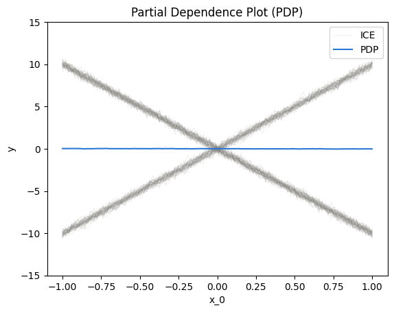
pdp = effector.PDP(X_test, predict)
pdp.plot(feature=0)
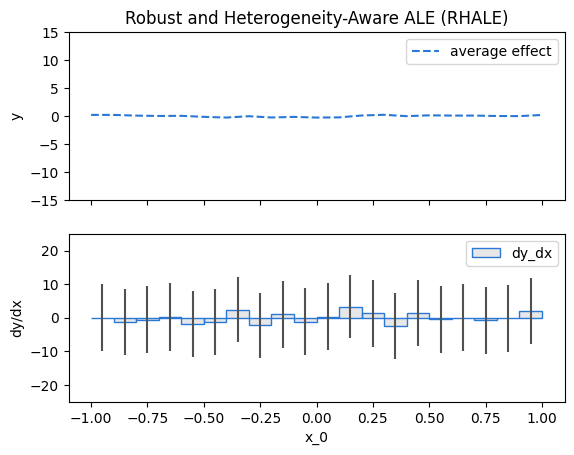
rhale = effector.RHALE(X_test, predict, jacobian)
rhale.plot(feature=0)
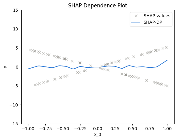
shapdp = effector.ShapDP(X_test, predict)
shapdp.plot(feature=0)
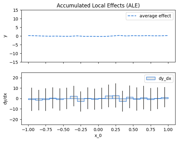
ale = effector.ALE(X_test, predict)
ale.plot(feature=0)
derpdp = effector.DerPDP(X_test, predict, jacobian)
derpdp.plot(feature=0)
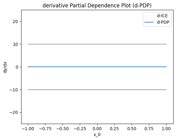
⚠️ Every mean curve above is flat, and the model is anything but. That
flat line is the average of a +10 slope and a -10 slope cancelling out.
The band around it is screaming; the line is not. That is what heterogeneity
is for, and why it is drawn by default.
The two arguments you will actually reach for
heterogeneity picks how the spread is drawn. Each method has its
native view, on by default:
| engine | default | other views |
|---|---|---|
PDP / DerPDP |
"ice" (per instance curves) |
"std" (a band), "std_err", False |
ALE / RHALE |
True (std band + per bin dy/dx bars) |
False |
ShapDP |
"shap_values" (the per instance scatter) |
"std", False |
centering picks the vertical anchor: False (raw), True
("zero_integral", zero mean), or "zero_start" (the curve starts at 0).
Centering moves the curve up or down; it never changes its shape or its
heterogeneity.
On real data
On the bike sharing rig, with the schema in the constructor, the same call renders in raw units and real level names:
pdp.plot("hr")
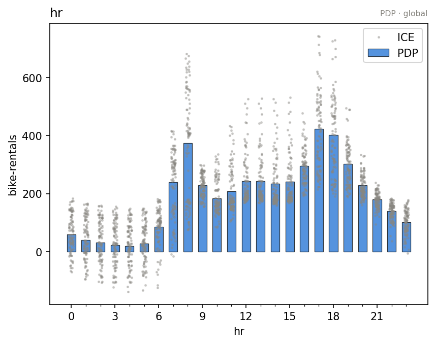
The mean curve shows the two commute peaks; the ICE cloud around the evening one is wide, and that spread is what the next pages will chase.
Plot inside a subregion
Every plot accepts mask= (a boolean (N,) array) or rule= (an
effector.Rule or a string). Rules speak your schema, level names included:
pdp.plot("hr", rule="workingday == no")
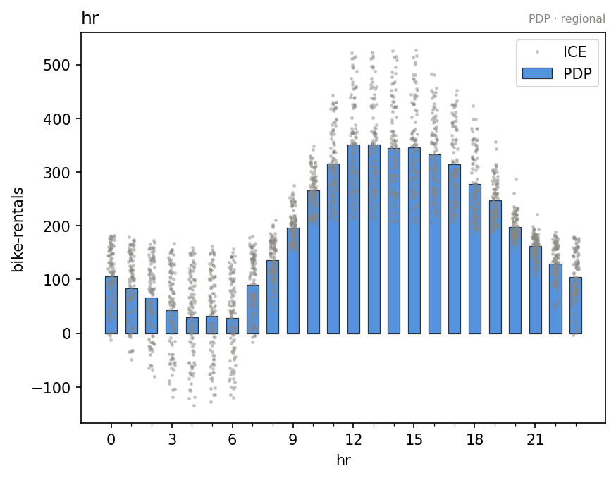
On non working days the commute peaks flatten into one midday dome. Same
cached effects, re summarized within the subregion, zero model calls.
This is the drill down you will use constantly once
find_regions hands you rules worth looking at.
Cosmetics
nof_points (grid resolution), nof_ice/nof_shap_values (how many
instances the heterogeneity view draws), scale_x/scale_y (display
scaling when you have no schema), y_limits/dy_limits, show_avg_output
(a horizontal line at the model's mean prediction), feature_label (axis
title override), and show_plot=False to script figures without a display.
👉 With a schema in the constructor, ticks, level
names, and units render correctly without any of the scale_* arguments.
Where to next
eval: the same numbers, without the picture- The interactive API: back to the guide's map
- Construct and fit: the previous page