The regional analysis
Description
The sixth component of effector's report: section 2 of
the HTML page and the partition trees of .show(). The selected
snapshot, feature by feature: trees, per leaf plots, and what a feature
without an accepted split shows instead.
Reading time
Approx. 6' to read.
What you see
Section 2 of the HTML page renders the final CALM: global effects
everywhere except the accepted splits. One subsection per plotted feature
(2.1 · hr, 2.2 · yr, ...), in descending snapshot importance, each opened
by three chips: importance, heterogeneity, regions.
In report.show(), the same information compresses to one ASCII tree per
accepted split, printed after the tables:
    hr 🔹 [id: 0 | heter: 0.48 | inst: 2000 | w: 1.00]
        workingday = no 🔹 [id: 1 | heter: 0.37 | inst: 614 | w: 0.31]
            temp < 4.50 🔹 [id: 2 | heter: 0.24 | inst: 248 | w: 0.12]
            temp ≥ 4.50 🔹 [id: 3 | heter: 0.32 | inst: 366 | w: 0.18]
        workingday = yes 🔹 [id: 4 | heter: 0.34 | inst: 1386 | w: 0.69]
            yr = 2011 🔹 [id: 5 | heter: 0.25 | inst: 696 | w: 0.35]
            yr = 2012 🔹 [id: 6 | heter: 0.32 | inst: 690 | w: 0.34]
Reading a tree
Chips read [id | heterogeneity | #instances | weight], and heterogeneity
drops as you walk down: 0.48 → 0.37 → 0.24. Every node is addressable by
its id; the leaves are the regions the report plots.
Rules speak your schema: workingday = no, yr = 2011, temp < 4.50 (°C,
not z scores), never x_6 ≤ -1.35. That is the
input layer paying off.
Why is the ranked table's heter different from the tree's root?
They answer different questions. The tree's root (0.48) is hr before
the split; the ranked features table (0.288) is
hr after it, averaged over the leaves. The gap between them is what
the split bought you.
A split feature's section
An accepted split feature opens with a caption that quotes its ledger row
(Split on temp, workingday, yr into 4 regions — worth +17.5% ...), then the
partition tree, then a grid of per leaf plots, one effect curve per
leaf:
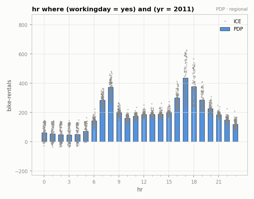
hr where workingday = yes and yr = 2011 |
hr where workingday = yes and yr = 2012 |
|---|---|
 |
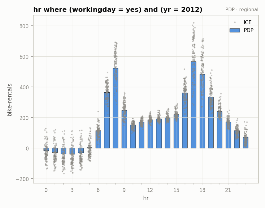 |
Each figure's title is its rule; the caption under it carries the stats
(heterogeneity 0.2530 · −48% vs global · n=3,463 for the 2011 leaf). Same
feature, same hours, and the two commute peaks ride visibly higher in 2012
than in 2011: that difference is exactly the spread the global plot buried
in its band.
👉 By default the y axes are shared across all figures of the page, so
levels are comparable at a glance; see share_y in
the configuration.
A feature without an accepted split
Everything else stays global: a Global effect figure, then a Regional effects note stating why there are no regional plots. Three variants:
| note | meaning |
|---|---|
heterogeneity below the threshold, find_regions was skipped |
the mean effect tells the whole story |
find_regions searched but no split passed |
heterogeneous, yet no candidate rule explains it |
| a split was found, but the decision sequence skips it | see the rejected splits; reproduce it with find_regions |
Nothing is drawn as if it had been accepted: a rejected split's regional plots are omitted on purpose, so the pictures and the ledger never disagree.
Two edge cases you may meet
A leaf whose rule pins the feature to a single value prints
the feature is constant inside this region — no curve to draw. And a
report rebuilt from to_dict() has no live effect to plot with: the per
leaf plots become a leaf statistics table (region, heterogeneity,
drop vs global, n), everything else renders as usual.
Where to next
- The global baseline: the next component
- effector's report: back to the guide's map
find_regions: grow these trees yourself